As a hobby project over the past few weeks, I’ve been training neural networks to predict the prices of cars in photographs. Anybody with some experience in ML can probably guess what I did, at least on a high level: I scraped terabytes of data from the internet and trained a neural network on it. However, I ended up learning more than I expected to along this journey. For example, this was the first time I’ve observed clear and somewhat surprising positive transfer across prediction tasks. In particular, I found that predicting additional details about each car (e.g. make and model) improved the accuracy of price predictions. Additionally, I learned a few things about file systems, specifically EXT4, that threw me off guard. And finally, I used AI-powered image editing to uncover some interesting behaviors of my trained classifier.
This project started off as a tweet a few months ago. I can’t remember exactly why I wanted this, but it was probably one of the many times that some exotic car caught my eye in the Bay Area. After tweeting out this idea, I didn’t actually consider implementing it for at least a month.
You might be thinking, “But wait! The app can’t possibly tell you exactly how much a car is worth from just one photo—there are just too many unknowns. Does the car actually work? Does it smell like mold on the inside? Is there some hidden dent not visible in the photo?” These are all valid points, but even though there are many unknowns, it’s often apparent to a human observer when a car looks expensive or cheap. Our model should be at least as good: it should be able to tell you a ballpark estimate of the price, and maybe even estimate the uncertainty of its own predictions.
The run-of-the-mill approach for building this kind of app is to 1) download a lot of car images with known prices from the internet, and 2) train a neural network to input an image and predict a price. Some readers may expect step 1 to be boring, while others might expect the exact same thing of step 2. I expected both steps to be boring and straightforward, but I learned some surprising lessons along the way. However, if that still doesn’t sound interesting to you, you can always skip to the results section to watch me have fun with a trained model.
Curating a Dataset
So let’s download millions of images of vehicles with known prices! This shouldn’t be too hard, since there’s tons of used car websites out there. I chose to use Kelley Blue Book (KBB)—not for any particular reason, but just because I’d heard of it before. It turned out to be pretty straightforward to scrape KBB because every listing had a unique integer ID, and all the IDs were predictably distributed in a somewhat narrow range. I ran my scraper for about two weeks, gathering about 500K listings and a total of 10 million images (note that each listing can contain multiple images of a single vehicle). During this time, I noticed that I was running low on disk space, so I added image downsampling/compression to my download script to avoid saving needlessly high-resolution images.
Then came my first surprise: despite having more than enough disk space, I was hitting a mysterious “No space left on device” error when writing images to disk. I quickly noticed an odd pattern: I could create a new file, write into it, or copy existing files, but I could not create files with particular names. After some Googling, I found out that this was a limitation of EXT4 when creating directories with millions of files in them. In particular, the file system maintains a fixed-size hash table for a directory, and when a particular hash table bucket fills up, the driver returns a “No space left on device” error for filenames that would go into that bucket. The fix was to disable this hash table, which was somewhat trivial and only took a few minutes.
And voila, no more I/O errors! However, now opening files by name took a long time—sometimes on the order of a 0.1 seconds—presumably because the file system had to re-scan the directory to look up each file. When training models later on, this ended up slowing down training to the extent that the GPU was barely utilized. To mitigate this, I built my own hash table on top of the file system using a pretty common approach. In particular, every image’s filename was already a hexadecimal hash, so I sorted the files into sub-directories based on the first two characters of their name. This way, I essentially created a hash table with 256 buckets, which seemed like enough to prevent the file system from being the bottleneck during scraping or data loading.
One thing I worried about was duplicate images in the dataset. For example, the same generic thumbnail image might be used every time a certain dealership lists a Nissan Altima for sale. While I’ve implemented fancy methods for dataset deduplication before (e.g. for DALL-E 2), I decided to go for a simpler approach to save compute and time. For each image, I computed a “perceptual hash” by downsampling the image to 16×16 and quantizing each color to a few bits, and then applied SHA256 to the quantized bitmap data. I then deleted all images whose exact hashes were repeated more than once. This ended up clearing out about 10% of the scraped images.
Once I had downloaded and deduplicated the dataset, I went through some of the images and saw that there was a lot of junk. By “junk”, I mean images that did not seem particularly useful for the task at hand. We want to classify photos of whole vehicles, not close-ups of wheels, dashboards, keys, etc. To remove these sorts of images from the dataset, I hand-labeled a few hundred good and bad images, and trained an SVM on top of CLIP features on this tiny dataset. I tuned the threshold of the SVM to have a false-negative rate under 1% to make sure almost all good (positive) data was kept in the dataset (at the expense of leaving in some bad data). This filtering ended up deleting about another 50% of the images.
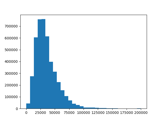
And with that, dataset curation was almost done. Notably, I scraped much more metadata than just prices and images. I also dumped the text description, year, make/model, odometer reading, colors, engine type, etc. Also, I created a few plots to understand how the data was distributed:
| Make / model | Ford F150 | Chevrolet Silverado | RAM 1500 | Jeep Wrangler | Ford Explorer | Nissan Rogue |
| % of the dataset | 3.75% | 3.41% | 2.11% | 1.88% | 1.69% | 1.64% |
Training a Model
Now that we have the dataset, it’s time to train a model! There are two more ingredients we need before we can start burning our GPUs: a training objective and a model architecture. For the training objective, I decided to frame the problem as a multi-class classification problem, and optimized the cross-entropy loss. In particular, instead of predicting an exact numerical price, the model predicts the probability that the price falls in a pre-defined set of ranges (e.g. the model can tell you “there is a 30% chance the price is between $10,000 and $15,000”). This setup forces the model to predict a probability distribution rather than just a single number. Among other things, this can help show how confident the model is in its prediction.
I tried training two different model architectures, both fine-tuned from pre-trained checkpoints. To start off strong with a near state-of-the-art model, I tried fine-tuning CLIP ViT-B/16. For a more nimble option, I also fine-tuned a MobileNetV2 that was pre-trained on ImageNet1K. Unlike the CLIP model, the MobileNetV2 is tiny (only a few megabytes) and runs very fast—even on a laptop CPU. I liked the idea of this model not only because it trained faster, but also because it would be easier to incorporate into an app or serve cheaply on a website. I did all of my training runs on my home PC, which has a single Titan X GPU with 12GB of VRAM.
In addition to the price range classification task, I also tried adding some auxiliary prediction tasks to the model. First, I added a separate linear output layer to estimate the median price as a single numerical value (to force the model to estimate the median and not the mean, I used the L1 loss). I also added an output layer for the make/model of the vehicle. Instead of predicting make and model independently, I treated the make/model pair as a class label. I kept 512 classes for this task, since this covered 98.5% of all vehicles, and added an additional “Unknown” class for the remaining listings. I also added an output layer for the manufacture year (as another multi-class task), since age can play a large role in the price of a car.
I expected the auxiliary prediction tasks to hurt performance on the main price range prediction task. After all, the extra tasks give the model more work to do, so it should struggle more with each individual task. To my surprise, this was not the case. When I added all of these auxiliary prediction tasks, the accuracy and cross-entropy loss for price range prediction actually improved faster and seemed to be converging to better values. This still leaves the question: which auxiliary losses contribute to the positive transfer? One data point I have is a buggy run, where I accidentally scaled the median price prediction layer incorrectly such that it was effectively unused. Even for this run, the positive transfer can be observed from the loss curves, indicating that the positive transfer mostly comes from predicting the make/model and year.
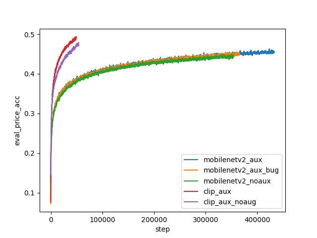
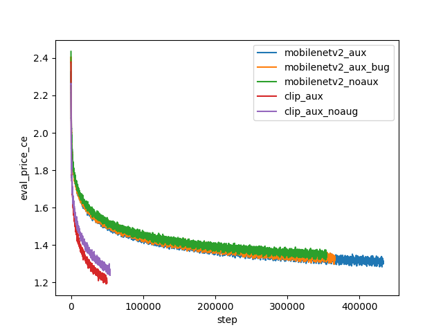
I’m not quite sure how to explain this surprising positive transfer. Perhaps prices are a very noisy signal, and adding more predictable variables helps learn more relevant features. Or perhaps nothing deep is going on at all, and adding more tasks is somehow equivalent to increasing the batch size or learning rate (these are two important hyperparameters that I did not have compute to tune). Regardless of the reason, having a bunch of auxiliary predictions is useful in and of itself, and can make the output of the model easier to interpret.
Looking at the above loss curves, you may be concerned that the accuracy is quite low (around 50% for the best checkpoint). However, it’s difficult to know if this is actually good or bad. Perhaps there is simply not enough information in single photos to infer the exact price of a car. One observation in support of this hypothesis is that the cross-entropy loss for make/model prediction was actually lower (around 0.5 nats) than the price range cross-entropy loss (around 1.2 nats). This means that, even though there are almost two orders of magnitude more make/model classes than price ranges, predicting the exact make/model is much easier than predicting the price. This makes sense: an image will usually be enough to tell what kind of car you are looking at, but won’t contain all of the hidden information (e.g. mileage) that you’d need to determine how expensive the car is.
Another thing you might have noticed from the loss curves is that none of these models have converged. This is not for any particularly good reason, except that I wanted to write this blog post before the end of the winter holidays. I will likely continue to train my best models until convergence, and may or may not update this post once I do.
Results
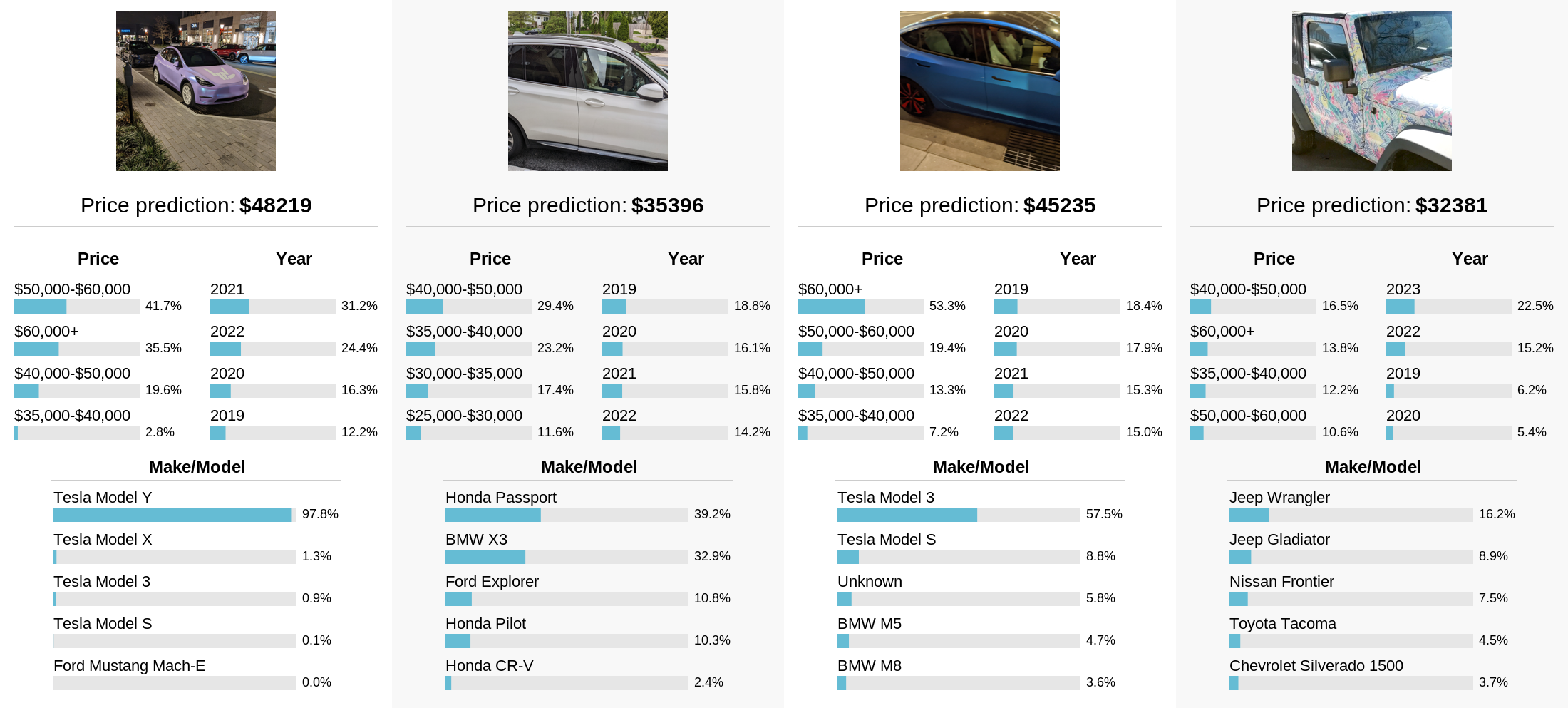
In this section, I will explore the capabilities and limitations of my smaller MobileNetV2-based model. While this model has worse accuracy than the fine-tuned CLIP model, it is much cheaper to run, and is likely what I would deploy if I turned this project into a real app. Overall, I was surprised how accurate and robust this small model was, and I had a lot of fun exploring it.
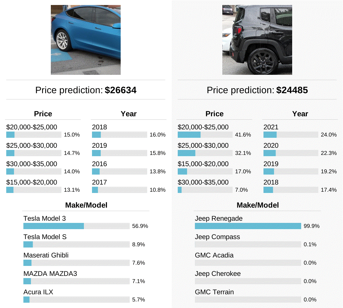
Starting off strong, I tested the model on photos of cars that I found in my camera roll. For at least three of these cars, I believe the make/model predictions are correct, and for one car I’m not sure what the correct answer should be. It’s interesting to note how well the model seems to work even for cars with unusual colors and patterns, which tend to dominate my camera roll.
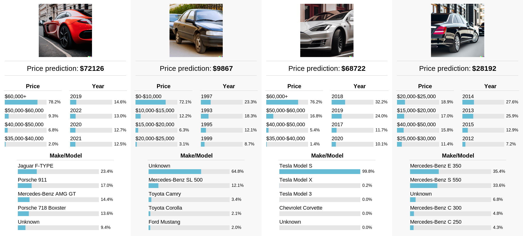
Of course, my personal photos aren’t very representative of what cars are out there. Let’s mix things up a bit by creating synthetic images of cars using DALL-E 2. I found it helpful to append “parked on the street” to the prompts to get a wider shot of each car. To me, all of the price predictions seem to make sense. Impressively, the model correctly predicts a “Tesla Model S” for the DALL-E 2 generation of a Tesla. The model also seems to predict that the “cheap car” is old.
So here’s a question: is the model just looking at the car itself, or is it looking at the surrounding context for more clues? For example, a car might be more likely to be expensive if it’s in a suburban neighborhood than if it seems to be in a shady abandoned lot. We can use DALL-E 2 “Edits” to evaluate exactly this. Here, I’ve taken a real photo of a car from my camera roll, used DALL-E 2 to remove the license plate, and then changed the background in various ways using another editing step:
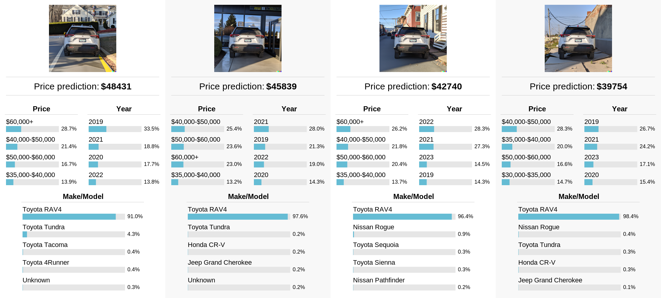
And voila! It appears that, even though the model predicts the same make/model for all of the images, the background can influence the predicted price by almost $10k! After seeing this result, I suddenly found new appreciation for what can be studied using AI tools to edit images. With these tools, it is easy to conduct intervention studies where some part of an image is changed in interpretable ways. This seems like a really neat way to probe small image classification models, and I wonder if anybody else is doing it.
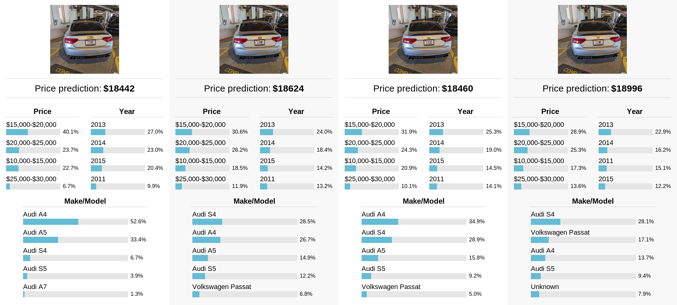
Here’s another question: is the model relying solely on the car logo to predict the make/model, or is it doing something more general? To study this, I took another photo of a car, edited the license plate, and then repeatedly re-generated different logos using DALL-E 2. The model appears to predict that the car is an Audi in every case, even though the logo is only a recognizable Audi logo in the first image.
For fun, let’s try one more experiment with DALL-E 2, where we generate out-of-distribution images of “cars”:
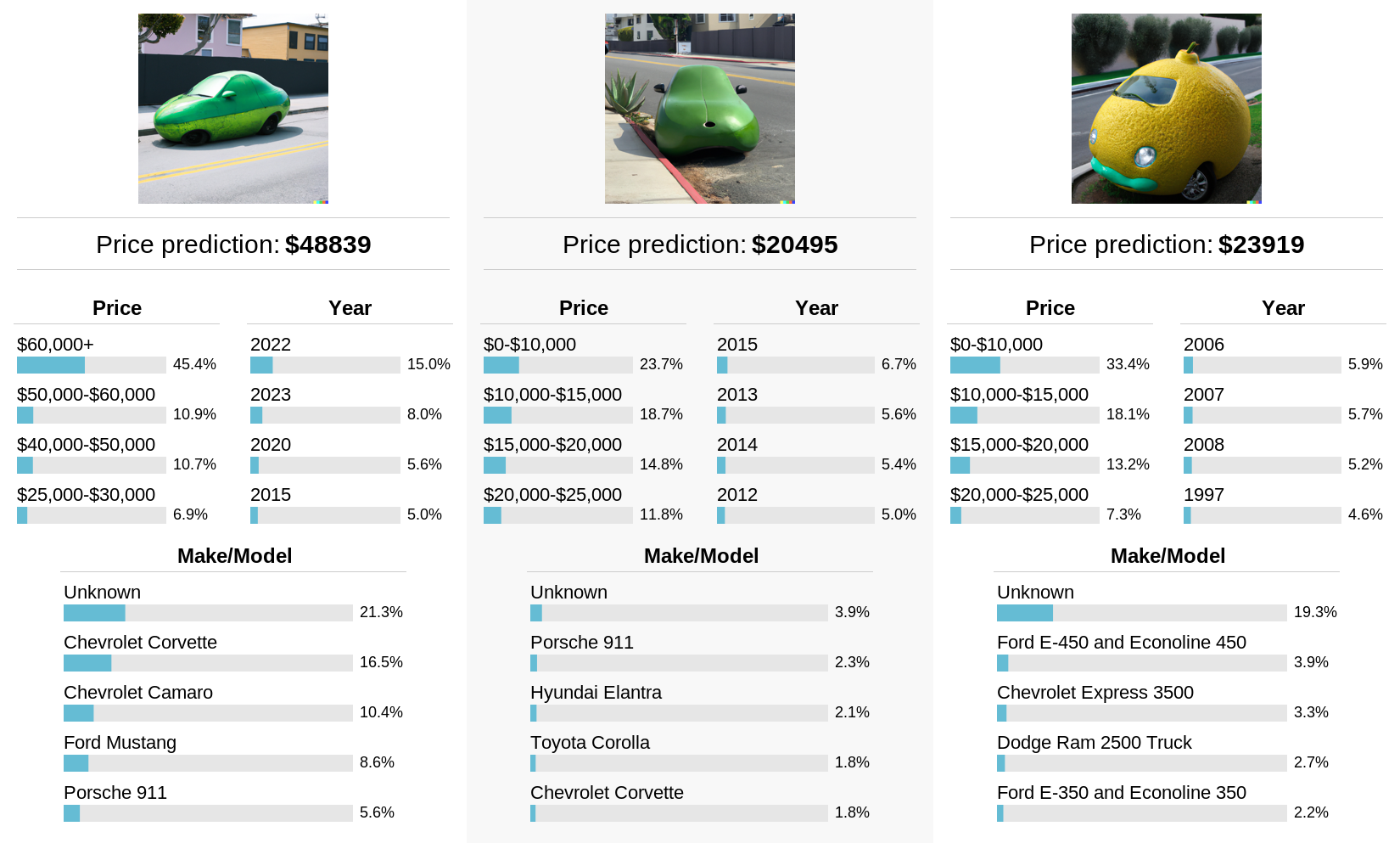
Happily, the model does not confidently claim to understand what kind of car these are. The price and year estimates are interesting, but I’m not sure how much to read into them.
In some of my earlier examples, the model correctly predicts the make/model of cars that are only partially visible in the photo. To study how far this can be pushed, I panned a crop along a side-view of two different cars to see how the model’s predictions changed as different parts of the car became visible. In these two examples, the model was most accurate when viewing the front or back of the car, but not when only the middle of the car was visible. Perhaps this is a shortcoming of the model, or perhaps automakers customize the front and back shapes of their car more than the sides. I’d be happy to hear other hypotheses as well!
Conclusion
In this post, I took you along with me as I scraped millions of online vehicle listings and trained models on the resulting data. In the process, I observed an unusual phenomenon where auxiliary losses actually improved the loss and accuracy of a classifier. Finally, I used AI-generated images to study the behavior of the resulting classifier, finding some interesting results.
After the fact, I realized that this project might be something others have already tried. After a brief online search, the closest project I found was this, which scraped only ~30k car listings (much smaller than my dataset of 500k). I also couldn’t find evidence of an image classifier trained on this data. I also found this paper which used a fairly small subset of the above dataset to predict the make/model out of a handful of classes; this still doesn’t seem particularly general or useful. After doing this research, I think my models might truly be the best or most general ones out there for what they do, but that wasn’t the main aim of the project.
The code for this project can be found on Github in the car-data repository. I also created a Gradio demo of the MobileNetV2 model, where you can upload your own images and see results.