In this post, I will present an algorithm that was able to compute an optimal tokenizer in some settings. This result is cool because optimal tokenization is theoretically intractable, but seems to be solvable in practice. My finding is very similar to various results on the Traveling Salesman Problem (TSP), where even difficult instances can be solved optimally using cutting-plane techniques.
I'll highlight that, while this result is cool, there are a few reasons that it isn't necessarily useful. First, the existing state of the art was already somewhat close to optimal (often within 1%). Second, even if a tokenizer is optimal on the training data, it may not generalize as well as other tokenizers when evaluated on held out test data. Finally, inefficient tokenizers are basically fine: you can pay for the cost of a less efficient tokenizer by slightly increasing your vocabulary size.
Despite the above caveats, I had a really fun time working on this project, and I hope others will be interested in pushing the frontier of this problem as well.
Background: Tokenizers
Frontier LLMs are typically trained on sequences of integers known as tokens. Each token refers to some sequence of bytes, and these byte sequences often correspond to common words. For example, in the GPT-5 tokenizer, the token 290 corresponds to the bytes “ the”, and 6602 corresponds to “ token”, so the text “ the token” can be encoded as the sequence [290, 6602].
The mapping from tokens to bytes, known as the “vocabulary”, is fixed before the LLM is even trained. Typically, we try to find a vocabulary that compresses a slice of training data. In particular, we would like to pick a vocabulary of a fixed size that minimizes the number of tokens required to encode the data. The dominant technique for finding such a vocabulary is byte-pair encoding (BPE), a decades-old greedy compression algorithm.
Tokenization as integer linear programming
In a recent paper, Tempus et al. connected tokenization to integer linear programming. The basic idea of their approach is to represent the entire dataset's tokenization as a set of integer variables.
In this formulation, there's a “color” variable for each possible vocabulary entry. In particular, we create one color variable for every unique substring of the dataset. A color variable is 1 if the corresponding byte sequence is in the vocabulary, or 0 otherwise. We add a single constraint to force the sum of color variables to equal the target vocabulary size.
A color corresponds to some sequence of bytes, but a given sequence of bytes may occur many times throughout the dataset. For each occurrence of a color, there's a separate “edge” variable. The edges work together to encode an actual tokenization of the dataset. If an edge is 1, then the edge's corresponding token is used in this particular place. The objective of our linear program is to minimize the sum of all the edge variables, i.e. the number of tokens used to encode our dataset.
For example, in the below picture, we tokenize the word “Queue” as the tokens [“Q”, “ue”, “ue”]. We could alternatively have tokenized it as [“Qu”, “e”, “ue”], but that is not the tokenization indicated by the current ILP solution, since the edge variables for the initial “Qu” and “e” edges are 0.
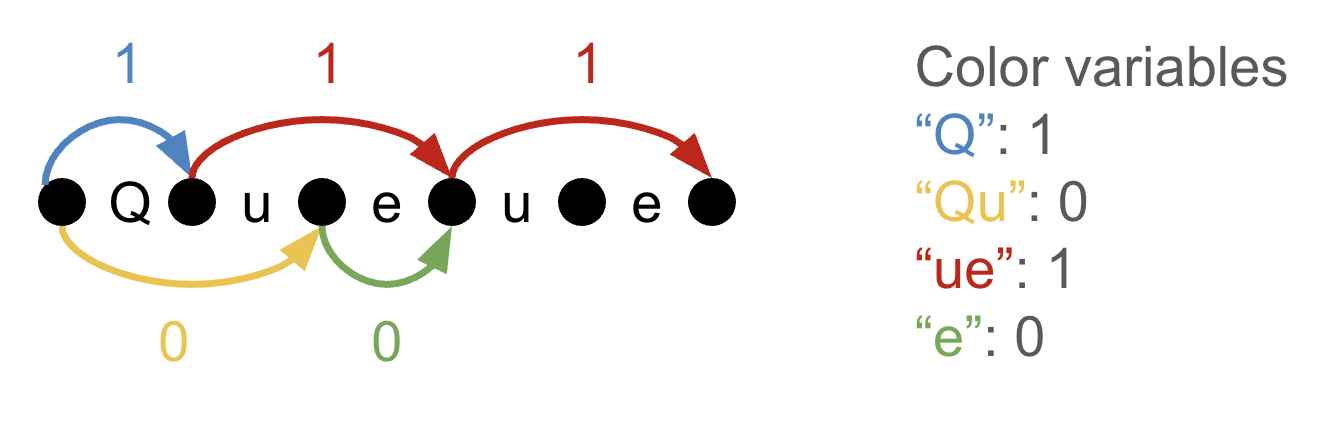
We constrain the LP in two ways. First, we can't use a token if it's not in the vocabulary. To this end, we constrain each edge variable to be less than or equal to its corresponding color variable. Second, we want to make sure that we tokenize the dataset in exactly one valid way. To this end, we add flow constraints: for each byte position in the dataset, we want the sum of edges flowing into this position to be equal to the sum of edges flowing out of this position, with the exception of the boundaries. For the first and last positions, we want the flow out or flow in to be 1. In an integer solution, you can see flow constraints as asserting the following: any point that an edge goes into must have an edge going out of it, except the first and last positions.
If all the variables were integral and constrained to [0, 1], then this linear program is enough to encode the optimal tokenization. However, since we cannot solve arbitrary integer linear programs efficiently, Tempus et al. relax the ILP to a continuous LP and solve this with a well-optimized solver.
The solution to the continuous LP is not generally integral. We can see an example of this below, where we have two superimposed tokenizations of the word “Queue”: either we encode it as [“Q”, “ue”, “ue”], or as [“Qu”, “e”, “ue”]. The problem with this solution is that our color variables sum to 2.5, but we've actually used four total colors, so we haven't actually found an optimal vocabulary of size 3. In general, we might end up with many more non-zero color variables than the actual vocabulary size we are targeting.
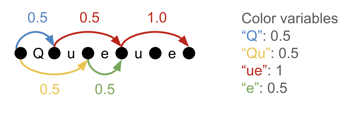
Tempus et al. propose to “round” the color variables in a few different ways, achieving an integral but suboptimal solution to the ILP. The solution to the continuous LP gives a lower bound on the optimal solution's token count, and the rounded tokenizer gives an upper bound.
One other caveat I should mention about this work: to make it tractable, we pretokenize the dataset (spit it into words) and merge repeated words (with corresponding weights in the objective based on how many times a word occurs). This drastically reduces the number of variables in the LP, but it does mean our solution is only “near optimal” under the pretokenizer. Today, I won't try to remove this restriction, but it would be an interesting direction for future work.
Cutting planes
I spent some time last year learning about the Traveling Salesman Problem (TSP), which can also be posed as an ILP. We can often use cutting planes to solve this ILP: first, we turn the ILP into a continuous LP, then add extra constraints until the optimal solution is integral. The constraints must be provably “valid”–that is, never violated for actual integer solutions. In theory, any ILP can be “turned into” a continuous LP with extra constraints, but the magical extra constraints may be intractable to find. TSP solvers use a number of heuristics to efficiently find such constraints in most practical cases. The authors of Corcorde (a TSP solver) wrote an entire book about techniques for finding useful cuts.
After reading Tempus et al., I wondered if we could apply cutting planes to the tokenization ILP. The method would work like this: first, solve the initial LP to get some lower and upper bound on the optimal tokenization; then, keep adding valid cuts to the LP and re-solving it to make these bounds closer and closer together–until they meet at the optimal solution.
It takes a lot of work and creativity to come up with “cut families” that might be useful for an ILP, so instead of banging my head against this myself, I set Codex on the task. At first, it found almost nothing–some of the cuts improved the LP bound a tiny bit, but most of the things it tried were surface-level word heuristics.
Then I tried another approach: brute force. A “cut” is some constraint that is satisfied by all integer solutions, but violated by the current fractional LP solution. We can find cuts by constructing an auxiliary linear program with one constraint for each possible integer solution, and optimizing it to maximize the violation of the fractional solution. We can't do this for the entire LP, since the number of rows blows up exponentially, but we can do it for small interesting “projections” of the LP. Codex proposed to look at all the variables in pairs or triplets of words with common fractional colors.
The above technique found really good cuts that improved the rounded tokenizer and raised the lower bound. However, this approach is really inefficient, since it involves solving (pretty large) auxiliary LPs for a huge number of word pairs. The next trick was to have Codex look at the actual cuts we were finding.
By looking at the brute force cuts, Codex discovered several cut templates that can be found more efficiently. The most effective family seems to be what Codex named “cycle constraints”. This technique finds pairs of overlapping fractional edges in the current LP solution. For example, we might find an overlapping (i.e. conflicting) pair of edges for colors A and B. We then find a few pairs that share common colors, such as another pair for colors B and C and another for C and A. We can then create a constraint out of the corresponding edge and color variables that is often violated by the continuous LP solution but never violated by a valid integral solution.
Finding the cycle of conflicting pairs AB, BC, CA can be done with a neat trick: construct a graph where the vertices are colors, and connect any pair of colors that overlap as fractional edges in the current solution. After you have this graph, run DFS to find cycles in it. Codex implemented this all autonomously, though I'm sure it's not an original trick.
Experimental setup
I was pretty hardware limited for this project, using only my Mac Studio and Mac mini. There aren't great GPU-accelerated LP solvers for this hardware, so I mainly leaned on the HiGHS single-core simplex solver. Sadly, I found that this solver sometimes stalls, especially for later iterations where we've applied a lot of (potentially degenerate) cuts.
To run experiments in a reasonable amount of time on this hardware, I studied single eBooks. I needed the LPs to remain small enough to solve on the CPU, so I kept the pretokenization approach of Tempus et al.
Finally, I adopted some heuristics from Tempus et al. to make the LP smaller, such as dropping color variables for substrings that appear less than 5 times. I also imposed a byte length limit on colors–in this case 16 bytes. I found that this made a difference compared to an 8-byte limit, where the optimal tokenization was slightly worse.
Results
I was able to find provably optimal tokenizers on at least a few toy problems. The one I am most proud of is an optimal tokenizer of vocab size 512 for the book Pride and Prejudice. The algorithm converged in about a dozen iterations, taking a bit over a day.
I tried increasing vocabulary size from 512 to 1024 on this same problem, and found that cycle constraints weren't enough on their own to find an optimal solution. The lower bound continued to move significantly after I added back other cut families, though my latest runs are still not finished. There are, without a doubt, other cut families to be discovered here as well, and some may even be necessary to solve the 1024-vocab problem.
Future work
At this point, the main bottleneck in my experiments is LP solve times. In many of my experiments, each LP solve can take between hours and days. I've tried a few solvers (HiGHS, the solver in SCIP, and OR-Tools PDLP), and all of them start to choke on my highly constrained LPs. My suspicion is that my cutting plane approach is creating degenerate LPs, and this could be a potential area for improvement.
Generally, I'd love to see someone continue to scale up this work to larger corpora. I doubt that the cut families I've explored are enough for harder problems, and there is surely a rich space of ideas to explore.
I'd also love to see somebody remove the pretokenizer. This currently makes the LPs quite large, since we don't get to merge repeated words. Removing the pretokenizer also eliminates the ability to use word-based cut strategies. For example, some of my cut strategies enumerate all of the valid integer solutions for each word, and then project these combinations into a subset of variables. These strategies need to be completely reframed for a “single huge word” dataset.
Conclusion
This was a neat project, and it was fun to see Codex do an entire research loop with just a small bit of guidance from me. I really hope to keep playing with it, but this is contingent on figuring out a solution to the slow LP problem.
The incredibly hacky Codex implementation of this project is available on Github. For reference, the optimal vocabulary for Pride and Prejudice that I found is here (note that the vocab is actually 510, because the codebase reserves two special tokens).