Sharing Streaming Services Across Households

Picture this: you settle in to enjoy a streaming session on your smart TV, only to be greeted by an error message instead of the usual lineup of movie titles. This error message states that your account—or rather, a family member’s account that you’ve been using—can no longer be accessed from this household.

While most people would see this as a cue to purchase a personal subscription, I saw it as a golden opportunity to learn more about computer networking. Thus, I set out to work around this restriction and document the process.

Along my journey, I learned a lot about the Linux networking stack and about OpenWrt, a popular Linux distribution for network routers. Someone with substantial networking experience will probably laugh at my ignorance throughout this blog post, but I’m hoping that most readers will be able to learn something just as I did.

The Problem

This scenario is familiar to many people: my parents subscribe to a bunch of streaming services, and I want to access these services without being on their home internet. Unfortunately, some streaming services are starting to wise up, checking that all the devices on an account are actually connected to the same network.

Since I periodically have access to my parents’ house, I’ll assume that I can put a Linux server behind their router and setup port forwarding to access this server remotely. Ideally, I’d like to tunnel internet traffic from my TV through this server, since this would mean all requests to streaming services would appear to originate from their home IP. If I could achieve this, it would effectively solve the problem.

Unfortunately, smart TVs are actually quite dumb most of the time, so I’ll assume that I can’t directly setup a VPN—or any other type of proxy—on the TV itself. The only thing I can configure on the TV is the WiFi network that it is connected to.

The Solution

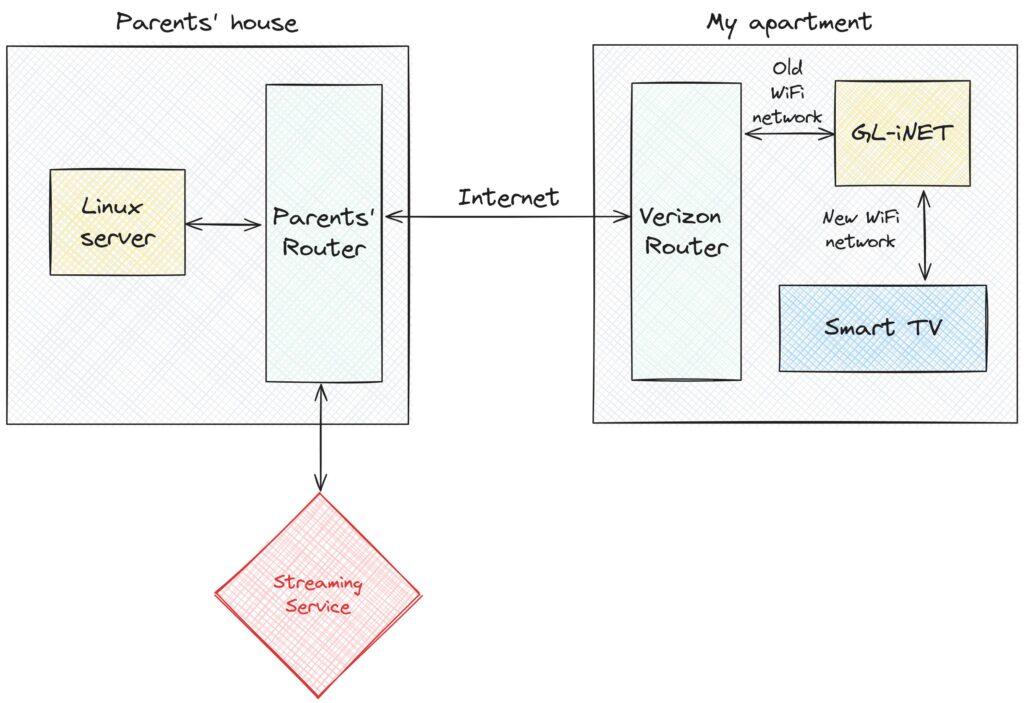
In short, I bought a cheap GL.iNet router and configured it to host a special WiFi network whose traffic is tunneled through my parents’ home network. Consequently, I can connect my TV to this WiFi network in my own apartment, and all of the TV’s internet traffic will appear to originate from my parents’ IP address. This bypasses the fact that the smart TV doesn’t understand anything about VPNs or proxies, since the GL.iNet can handle this.

The following diagram shows the resulting connectivity graph. On the right, I show that the GL.iNet connects to my existing WiFi network, and also exposes a new WiFi network for the smart TV to connect to. In this setup, nothing in my apartment connects to the streaming service directly. Instead, the Linux server at my parents house talks both to the streaming service and to my apartment, essentially turning my parents’ house into a proxy.

A connectivity diagram of a network with two boxes. On the right is a box labeled "My apartment", and on the left is one labeled "Parents' house". There are arrows showing connections between machines in both locations, including a linux server, a router in both homes, a smart TV, and a GL-iNet

This might sound pretty straightforward, and I believed that it would be when I started this project. However, it turned out to be pretty frustrating, requiring hours of time debugging and googling before I was able to get everything right. There were a few things that made this difficult. Most importantly, I started with only a rudimentary understanding of how the Linux kernel routes network packets, and this resulted in a lot of initial confusion. Additionally, I hadn’t used OpenWrt before, so I was starting from square one when it came to working with configuration files on the GL.iNet. More generally, I chose to use a lot of tools that I’d never used before, and this created a pretty steep learning curve.

I’ll split this post up into a few parts, describing the different steps I passed through on the path to my final setup. Roughly, I’ll talk about these three things:

  1. Setting up a VPN, in this case WireGuard, to connect my GL.iNet to the server at my parents’ house.
  2. The initial configuration I tried on the GL.iNet to tunnel traffic, and the hacky solution that eventually worked.
  3. How I cleaned up the routing table on the GL.iNet to isolate tunneling to a single “guest” WiFi network.

Setting up WireGuard

This is the part that I actually got mostly right on the first try. My goal was to create a VPN between the GL.iNet and the server at my parents’ house. I had heard good things about WireGuard, so I started by following this lovely DigitalOcean tutorial. After following this tutorial, I ended up with a WireGuard configuration on the server that looked like this:

A wireguard configuration on a Linux machine. There are red boxes over private and public keys and remote IP addresses.

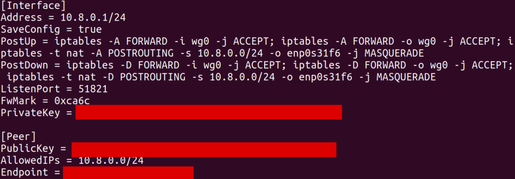
This configuration creates an interface (in my case, wg0) with a local IP address 10.8.0.1. The [Peer] section allows another WireGuard client (which will be the GL.iNet) to connect to this server and register itself with some other IP address 10.8.0.x (in my case, 10.8.0.2).

As far as I understand it, the iptables commands in PostUp setup NAT’ing, where 10.8.0.1 will act as a “router” of its own. In particular, this server is connected to my parents’ network over an Ethernet interface enp0s31f6. It has its own IP, something like 192.168.1.123, and can access the internet by sending packets over this interface with 192.168.1.123 as the source IP. What we’d like is for traffic from other clients on the WireGuard interface to be routed through enp0s31f6 so that they can access the internet through this same Ethernet connection. The MASQUERADE rule does this. In particular, when wg0 receives a packet from some other IP (e.g. 10.8.0.2) which is destined for some external IP (e.g. 8.8.8.8), some module in the kernel will know to rewrite the source IP in the packet to its own local IP (192.168.1.123) and send it over enp0s31f6. Furthermore, when it receives response packets on enp0s31f6 for this same logical connection (presumably identified by port and remote address), it will forward them back to 10.8.0.2 on wg0.

Unfortunately, the tutorial I was following did not describe how to setup WireGuard on an OpenWrt router. To achieve this, I basically mashed together several examples from internet forums to create the following client configuration on the GL.iNet:

An OpenWrt UCI configuration block for a WireGuard client. There are red boxes hiding private and public keys as well as remote IP addresses.

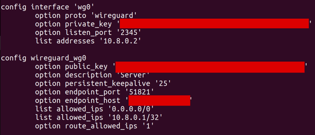
One important point, which took me a while to discover, is that allowed_ips has to include 0.0.0.0/0. Without this, I wasn’t able to send packets destined for arbitrary IP addresses over the wg0 interface (well, I could send them, but they’d silently get dropped). In retrospect, route_allowed_ips doesn’t really need to be enabled, since the default route it ended up creating didn’t work (which we’ll get to later). Also note that the endpoint_host is set to my parents’ remote IP, and I had to forward port 51821 on their router to my server.

With this configuration in place, I could run the wg command on the GL.iNet and find that the VPN was connected properly. I was also able to use the address 10.8.0.1 to ping and SSH into my server from the GL.iNet, indicating that things were mostly wired up correctly.

The output of the wg WireGuard command on a GL.iNet router. Private information is hidden by red boxes.

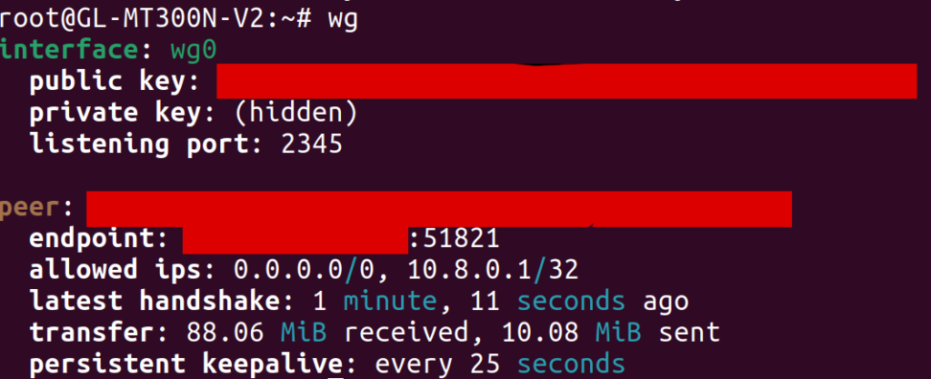
One hiccup I ran into was that, at first, I hadn’t added a [Peer] section to the WireGuard config on my server. As a result, the client was unable to connect to it, but the output of wg on the GL.iNet still looked basically the same (except that the latest handshake line was missing). As someone who hadn’t used WireGuard before, it was tough for me to tell that anything was wrong. In my opinion, WireGuard should make it more obvious when it hasn’t ever been able to reach a peer, since I wasn’t sure what to look for to see where things were broken.

Routing Traffic over WireGuard

After setting up WireGuard, I SSH’d into the GL.iNet and ran traceroute google.com to see if traffic was being routed through my parents’ home network. Surprisingly, traffic was still being routed directly over my apartments’ wireless network (the router of which was at 192.168.1.1), bypassing WireGuard altogether:

The output of a traceroute to google.com, with the first hop hitting 192.168.1.1. Some addresses are hidden by red boxes.

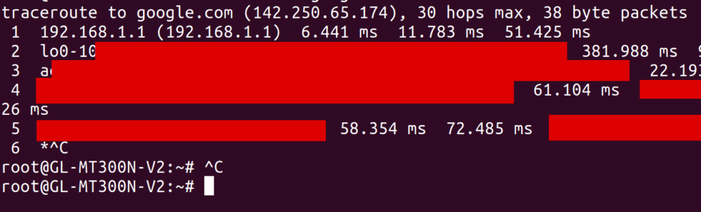
At the time, I had no idea why this would be the case. I understood a bit about routing tables, so I looked at the output of ip route show. I saw a default route over wg0 (presumably created by the WireGuard route_allowed_ips flag), and a second one via my apartment’s WiFi (via the apcli0 device).

The output of the command `ip route show`, with a remote IP address censored by a red box.

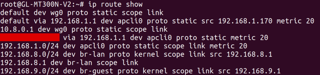
I tried deleting the latter default route, leaving only the route over wg0. To my dismay, I found that it made no difference: the output of traceroute was unchanged! While I later discovered what was actually going on, I’ll tell this story in chronological order by first describing a ridiculous workaround that I found to this problem.

I noticed that I could create specific routes to forward individual destination IP addresses through wg0, and these routes did seem to work. For example, I added a route for my personal website via the command

# route add -host 198.74.59.95 dev wg0

and then all traffic to 198.74.59.95 was correctly routed through WireGuard. I suspected that this had to do with the way the routing table prioritizes routes. In particular, more specific routes take higher precedence than general routes. The routes I was creating were about as specific as it gets, since they were scoped to single addresses, so of course they’d be the highest priority.

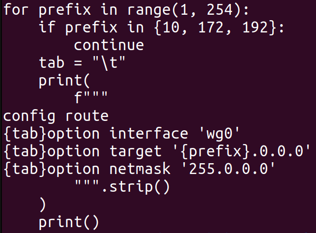
At this point, I was pretty sure that I could route all traffic over wg0 by creating a route for all 2^32 IPv4 addresses. However, I didn’t want to test how the Linux kernel would handle this kind of ridiculousness, so I instead created roughly 256 routes, each forwarding x.0.0.0/8 over wg0. I figured out how to do this via OpenWrt’s UCI configuration files, and dumped the output of the following Python script at the end of /etc/config/network:

This is Python code which creates many routes in an OpenWrt UCI configuration file.

After setting up this configuration, I indeed saw traceroute doing the right thing when accessing external IP addresses:

The output of a traceroute to google.com, where the first hop is 10.8.0.1 and the second is 192.168.1.1. Further hops are censored out by red boxes.

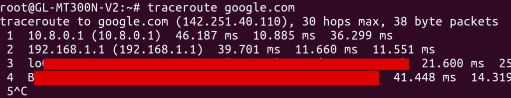
Note from this output that the traffic first hops to 10.8.0.1 and then to 192.168.1.1. You might be concerned that traffic is still going over my apartments’ router at 192.168.1.1, but worry not. Just to maximize confusion, my parents’ router also has the local IP address 192.168.1.1, and that’s the hop that we are seeing in this case.

Now that traffic on the GL.iNet was being routed over the VPN, I figured I’d try setting up an actual WiFi network. When I first configured the network on the GL.iNet, I connected to it from my laptop and found that traffic couldn’t get through to the internet at all. I ended up needing the following firewall configuration (in /etc/config/firewall) on the GL.iNet in order to pass traffic correctly from the “guest” WiFi network to the WireGuard interface:

An OpenWrt UCI configuration file defining firewall zones for a guest WiFi network and a wireguard device.

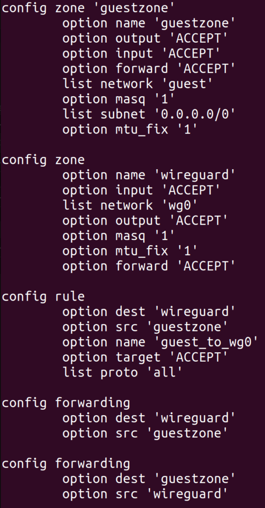
It took an embarrassingly long time to get this config right, and each time I changed it, I had to wait a minute or two for various services on the GL.iNet to restart. Most troubling of all was the mtu_fix flag, which took me about two hours to discover. Before I set that flag, I was already able to access most websites from the new WiFi network, and they were correctly tunneled through my parents’ home network. However, some websites did not load at all, and curl -v typically showed that the connection was stalling during the TLS handshake.

The output of `curl -v` to google.com with a red arrow pointing to a particular line, saying "Froze here".

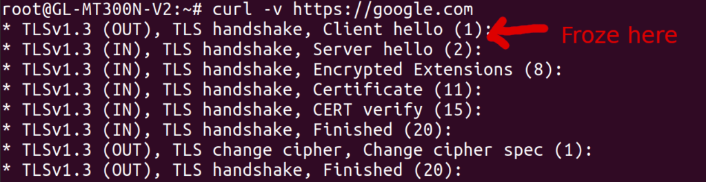
I found this thread after some googling, which suggested an MTU issue. The MTU is essentially the maximum size of a packet that can pass through a network device. For most common networks, this seems to default to 1500, but for the WireGuard interface on my GL.iNet, it was 1420 (as shown by ip addr):

An `ip addr` entry describing a wg0 interface. Shows that the MTU of the interface is 1420.

This isn’t a mistake, but rather a side effect of the fact that WireGuard wraps packets with some extra headers, which apparently take up 80 bytes. However, my laptop believed that the WiFi network had an MTU of 1500, as shown by ip addr:

The output of an `ip addr` command with an arrow pointing to the MTU of 1500.

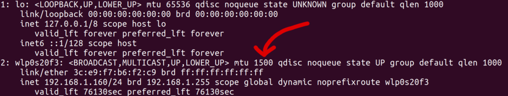
To test the hypothesis that mismatching MTUs were causing the stalled connections, I manually overrode the MTU of the wlp0s20f3 interface on my laptop to a smaller value, using the command

# sudo ip link set mtu 1300 wlp0s20f3

And presto, suddenly all websites loaded without any problems! Of course, I couldn’t manually override the MTU of network interfaces on my smart TV, so I needed another solution. After reading about path MTU discovery, I noticed a technique called MSS clamping, where a router in the network path modifies the “maximum segment size” field of TCP packets to fill in the minimum MTU of the devices it knows about. I was about to implement this by hand (perhaps with iptables or even eBPF) when I noticed the mtu_fix field in the OpenWrt firewall config documentation:

A screenshot of OpenWrt UCI documentation, with the mtu_fix field highlighted by a red circle.

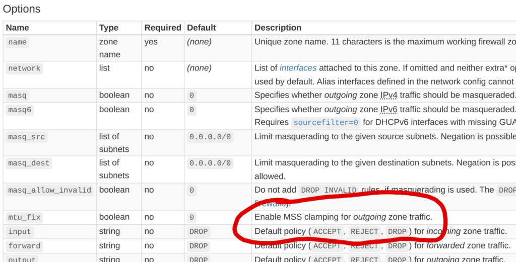
I enabled this option, and boom, connections worked even without manually overriding the MTU of my network interface! I still don’t know what will happen when using non-TCP protocols like QUIC, and I do slightly worry about that. In the future, I’d like to figure out a way to make my VPN support larger packets without constraining the MTU, even if it does mean creating more packet fragmentation.

Cleaning up the Routing Table

While my current solution did technically solve the problem I had set out to solve, it had two downsides that I wanted to address:

  1. It was messy. I now had over 256 routing table entries, and it felt like this shouldn’t be necessary. Ideally, I should be able to use a single routing table entry to forward all traffic over wg0. It was currently a mystery why this did not work as expected.
  2. The wg0 routes were applied globally. Ideally, these routes would only be applied to traffic coming from the special WiFi network itself. This might be a problem if, for example, I wanted to expose two WiFi networks from the GL.iNet: one which acts as a normal repeater, and another one that tunnels traffic through my parents’ house. With my current setup, this would be impossible.

To solve the first problem, I had to learn more about how Linux routes IP traffic. Up until now, I only knew about the “main” routing table, which can be shown and manipulated with the deprecated route command, or with the ip route command without a table argument. A routing table itself only uses the destination IP address of a packet to determine which device (and gateway) to send that packet to. This isn’t very flexible, since it doesn’t allow us to consider the source address or other attributes of the packet.

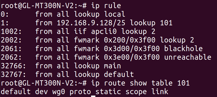
To create more complex routing rules, we can use the ip rule command to configure Linux’s routing policy database (RPDB). This lets us use various information about each packet to determine which routing table(s) to look at. To see all of the rules in the RPDB, we can use the ip rule command. Here was the output on the GL.iNet:

The output of an `ip rule` command, showing several rules including ones pointing to table 2.

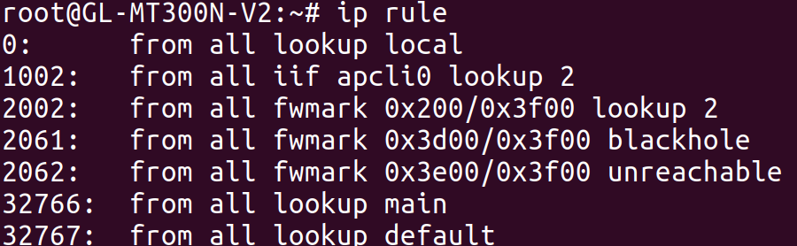
By default, there will only be three tables (local, main, and default) and one rule for each of them. In the output above, we see more rules, including this one:

from all fwmark 0x200/0x3f00 lookup 2

This rule points to table 2 (a different table than any of the built-in ones), and matches all traffic where fwmark & 0x3f00 == 0x200. Apparently, fwmark (the “firewall mark”) is an additional number associated with each packet that can be modified by firewall rules. I can’t claim to understand what sets this particular firewall mark on packets coming through this particular system, and I’d definitely like to understand more about this. Regardless, let’s take a look at table 2, since that’s where this rule points to:

The output of `ip route show table 2`, revealing a default route pointing to 192.168.1.1.

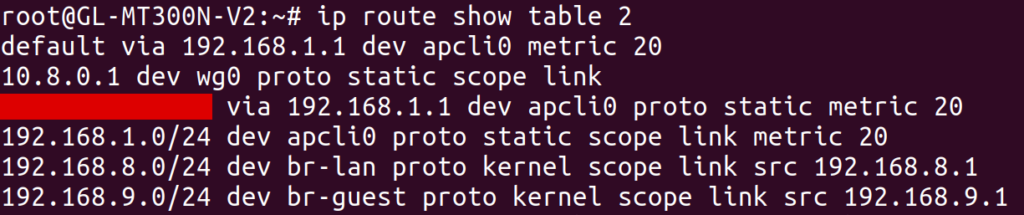
Aha! This routing table contains its own default route over apcli0 through 192.168.1.1 (my apartment’s router). This is a different default route than the one we saw earlier, which had been in the main table. Out of curiosity, I tried deleting all of my earlier custom routing rules, and additionally deleted the table 2 rule with:

# ip rule del fwmark 0x200/0x3f00 lookup 2

After deleting this rule, the default wg0 route from the main routing table took effect, automatically routing all traffic over the VPN! So this at least solved one mystery: I had only been looking at the main routing table, but there was a higher-priority rule that was directing traffic to a different default route than the one I was looking at. Granted, I still don’t know what created table 2 or the corresponding rules pointing to it, and some preliminary grep’ing of /etc didn’t yield anything particularly informative. I’d be curious to know if anybody else knows the answer.

Moving onto the second problem, I leveraged my newfound knowledge of policy routing to narrow the scope of the VPN route. In particular, I only wanted to route traffic over the VPN if it was coming from machines on a guest WiFi network. Since I configured my GL.iNet’s guest WiFi network to assign IP addresses in the range 192.168.9.128 through 192.168.9.254, all I needed to do was define a routing rule to route traffic from this range over the wg0 interface. I started by testing this idea with the ip command, and then created a UCI config for it in /etc/config/network:

An OpenWrt UCI config file containing both a `config rule` and a `config route`. These operate on table 101, and make a select range of source IP addresses get forwarded to the wg0 interface.

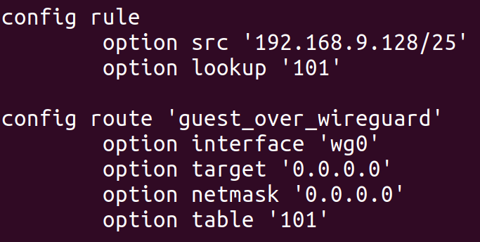
This configuration adds a route to table 101 (an arbitrary number I selected) with a single entry: a default route over wg0. The config rule section creates a rule to point all traffic coming from IPs on the guest WiFi network to this new table. After doing so, we can see the effects with the ip command:

The output of `ip rule` and `ip route` showing the result of a new routing rule which is scoped to a select range of IP addresses and routes this traffic to the wg0 interface.

The end result is that traffic from the guest WiFi network is routed over wg0, but traffic from the GL.iNet itself, or from other WiFi networks exposed by the GL.iNet, is not. I actually tested this by exposing a second WiFi network from the GL.iNet and verifying that its traffic was not routed through the VPN. This was more of a victory lap than anything else, to verify that I actually understood what was going on.

Conclusion

After going through this saga, I decided that it was time to set this project down for a while. I had a working setup, and ended up learning a lot more than I intended.

However, I was left with a few unanswered questions at the end of the process:

  • Is there a better alternative to MSS clamping? And what happens for other protocols like QUIC? And perhaps more importantly, why isn’t standard MTU path discovery working in the first place?
  • What created the routing table 2 in the first place, and those two rules pointing to it? And what is setting the 0x200 fwmark that triggers the routing rule in the first place?
  • Why is the network so slow? At the moment, it’s only able to achieve 5-10 Mb/s, which is much slower than my personal network or my parents’ network. I think this may be a limitation of the GL.iNet itself, since the speed isn’t much better even without tunneling through the VPN.

Even though I reached my goal, there’s more work that I could have done. At the moment, I don’t do anything to tunnel DNS traffic, so my apartment’s ISP still happens to determine the DNS server that my TV uses. I don’t think streaming services will notice this, but it could be worth fixing even if just for privacy reasons while traveling with my GL.iNet in the future.

I spent about $30 on the GL.iNet, which is enough to purchase a few months of any reasonably-priced streaming service. While it was probably not worth the effort from a monetary standpoint, I still think it was worth it 100 times over when factoring in the learning I got to do along the way.

I’ll leave you with the observation that this project didn’t require writing any real code! It’s unusual for me to spend so much time working on something that really boils down to writing the right config files. Perhaps that’s a testament to how powerful the Linux kernel (and other existing software) is when it comes to networking. Or, perhaps, it’s a sign that what I did wasn’t really that interesting or impressive at all.

Representing 3D Models as Decision Trees

As a hobby project over the past few months, I’ve been exploring a new way to represent 3D models. There are already plenty of 3D representations—from polygon meshes to neural radiance fields—but each option has its own set of trade-offs: some are more efficient to render, some are easier to modify, and some are cheaper to store. My goal with this project was to explore a new option with a new set of trade-offs.

The technique I will describe is storage-efficient, supports real-time rendering, and allows straightforward shape simplification. While the method isn’t suitable for every application, I can imagine scenarios where it could be useful. Either way, I think it could make a good addition to any 3D developer’s toolbox, or at least lead to other interesting ideas.

Representing Shapes as Decision Trees

The crux of this project is to represent 3D occupancy functions as oblique decision trees. It’s totally okay if you don’t understand what this means yet! I’ll break it down in this section, starting by describing decision trees in general, and then moving towards my specific method. You may want to skip this section if you are already familiar with occupancy functions and oblique decision trees.

In general, a decision tree takes an input and makes a prediction based on attributes of this input. For example, here’s a decision tree which predicts whether or not I will eat a given piece of food:

In this case, a food item is the input, and the output is a prediction “yes” or “no”. To make a decision, we start at the top (“Is it sweet?”) and follow the left or right arrow depending on the answer to this question. We repeat this process until we end up at a leaf (one of the triangles) which contains the final prediction. We refer to the yellow boxes as branches, since they branch off into multiple paths.

This picture might look intuitive, but what does it have to do with 3D shapes? To understand the answer, you might have to change how you think about shapes in general. We typically describe shapes by composing other shapes. For example, you might say that a person has a spherical head at the top, a wide rectangular torso underneath, and then two long cylindrical legs. However, you can also define a shape as an answer to the question “is this point inside the shape?” for every point in space. For example, a circle can be defined as every point \((x, y)\) such that \(x^2 + y^2 <= 1\). This is called an occupancy function, and it looks more like something we could do with a tree. In this setup, the input to the tree is a coordinate, and the output is a boolean (true or false) indicating whether or not the coordinate is contained within the shape.

To give a simple concrete example, let’s try to represent a 2-dimensional unit square as a decision tree. The input will be an \((x, y)\) coordinate and the output will be true or false. But what will the branches look like? Thinking back to the food example, we were able to ask questions about the food item, such as “Is it sweet?”. What kinds of yes/no questions can we ask about an \((x, y)\) coordinate? For now, let’s restrict ourselves to inequalities along a single axis. With this in mind, we might arrive at the following tree:

This tree might seem more complicated than it needs to be, due to our restriction on the types of branches we can use. In particular, we needed four branches just to express this simple function, while the whole tree could be reduced to a single branch with the predicate

$$(-1 <= x <= 1) \land (-1 <= y <= 1)$$

However, we’ll find later on that restricting the space of allowed branches makes these trees easier to render. More broadly, though, the power of decision trees is that their individual branches can be simple, but multiple steps of branching can lead to complex behavior.

With that being said, we will make our branches a little more powerful. In particular, we will use oblique decision trees, where the decision at each branch is based on a linear inequality of the input coordinates. In three dimensions, this means that each branch is of the form \(ax + by + cz < w\) where \(a, b, c\), and \(w\) are free variables. Geometrically, each branch divides the space across a plane, and \(<a, b, c>\) is the normal direction of the plane.

Why Decision Trees?

Perhaps the nicest property of decision trees is that they can make predictions quickly. For example, consider the game “20 questions”, where a decision tree that can identify any object with just 20 branches. This could be a really nice property for a 3D representation, especially for tasks like rendering and collision detection that we want to perform in real time.

Another nice property of decision trees is that they tend to be pretty small. Unlike neural networks, which are typically trained as large, fixed pools of parameters, decision trees can adapt their structure to the underlying data. In the context of 3D representations, this might mean that our trees could automatically adapt their size and complexity to each 3D shape. This sounds like a great way to save space for video games or other 3D-heavy applications!

Despite these benefits, pure decision trees aren’t very popular in machine learning because they are prone to overfitting (note that decision trees are still popular, but they are typically used in ensembles). Overfitting means that, while a tree might perfectly fit the set of examples it was built for, it might not generalize well to new unseen examples. While overfitting might be an issue in machine learning, it’s actually a good feature for representing 3D shapes. If we already know the shape we want to represent, we can create an infinite dataset of input points and corresponding outputs. We need not worry about overfitting—all we care about is fitting the (infinite) training data with a small, efficient tree.

Building Decision Trees

Even if decision trees are a reasonable way to represent 3D shapes, I doubt 3D artists would want to manually write out hundreds of decision branches to describe an object. Ideally, we would like to automatically create decision trees from known, existing 3D shapes. Luckily, there are many popular algorithms that are easy to adapt to this use case. In this project, I build on two such algorithms:

  • ID3 builds decision trees greedily, starting at the root node and working from the top down. In this algorithm, we create a branch by measuring the entropy of all possible splits, and choose the split with the most information gain.
  • Tree Alternating Optimization (TAO) refines a tree by optimizing each branch using a linear classification technique like support vector machines. This is a relatively new approach, and its main benefit is that it can help find better split directions for oblique decision trees.

Both of these approaches require a dataset of input-output pairs. Luckily, if we already have a known 3D model that we would like to encode as a tree, it is trivial to generate such a dataset. All we need to do is sample random points in space and evaluate whether each point is inside the 3D model. I encoded existing triangle meshes in all of my experiments, so I was able to use my model3d framework to detect whether points were inside or outside of the meshes.

Unlike in most machine learning scenarios, here we have the unique opportunity to leverage an infinite dataset. To make ID3 and TAO leverage infinite data, we can sample more data whenever it is “running low”. For example, we might start ID3 with 50,000 examples, but after making eight splits, we will be in a subspace where there are only \(50,000/2^8 = 195\) examples on average from this initial dataset. Whenever we don’t have enough examples to confidently keep building a sub-tree, we can sample more points in the current branch. In an oblique decision tree, the subspace of points that end up at a particular branch is defined by a convex polytope, and we can sample new points inside this polytope using a hit-and-run method. We can use a similar approach for TAO to ensure there are always enough examples to get a reasonable fit at every level of the tree.

Decision trees are often applied to categorical feature spaces where there are a small number of possible values for each feature. Our 3D case is very different, since we only have three dimensions, but we want to consider an infinite number of splits (i.e. all possible directions). For ID3, we have no choice but to explore a finite subset of these directions. In my code, I opted to use the vertices of an icosphere to get a fairly uniform set of directions to search over. After greedily selecting an optimal direction from this set, my ID3 implementation then generates a set of mutated directions and also searches this narrower set. This way, we can explore a large but finite space of directions when building the tree. Luckily, TAO comes to the rescue even further by allowing us to refine the tree using a continuous optimization method like gradient descent. This way, we can technically find any split direction, not just one choice from a finite set of options.

Real-time Rendering

So now we can create trees from arbitrary 3D models, but so far we have no way to visualize what we have created. What we really want to do is render the 3D object as an image, ideally fast enough that we could even create videos of the object in real time. In this section, I’ll show that we can, in fact, render our decision trees efficiently. This will also let us see, for the first time, what we can actually represent with this approach.

Before I implemented efficient tree rendering, I used a more naive approach to make sure my tree learning algorithms were working correctly. Since our decision trees represent a field of occupancy values, we can turn the tree back into a triangle mesh using a method like marching cubes, and then render this mesh using a standard rendering pipeline. This was great for quick prototyping and debugging, but it was expensive to run and often missed fine details and edges of the surface. Moreover, this approach defeats the purpose of representing the 3D model as a tree in the first place—we might as well have stuck with meshes!

Fortunately, there is another way to render our trees without ever converting them into a different representation. This technique is based on ray casting, where each pixel in the rendered image corresponds to a different linear ray shooting out from the camera. In particular, each ray starts at the camera origin \(\vec{o}\), and shoots in a direction \(\vec{d}\) that is specific to this pixel. We can represent this ray as a function \(\vec{r}(t) = \vec{o}+t\vec{d}\) where \(t \ge 0\) increases as we move farther from the camera along the ray. If the ray hits the object, we can then figure out what color the corresponding pixel should be from properties of the object’s surface at the point of collision. If the ray misses the object and shoots off into infinity, then the pixel is transparent.

To use ray casting, we just need to figure out where a ray collides with our decision tree. A naive approach would be to start at \(t=0\) and gradually increase \(t\) by small increments while repeatedly checking if the tree returns true at the point \(\vec{r}(t)\). However, this approach would be expensive, and it’s possible we could completely miss an intersection if we took too large of a step. Really, this approach is completely dependent on how much we increase \(t\) as we cast the ray. On one hand, we don’t want to take too small of a step: it would be inefficient to keep increasing \(t\) by 0.001 if none of the decision branches will change until \(t\) is increased by 0.1. On the other hand, we don’t want to completely miss collisions: it would be bad to increase \(t\) by 0.1 if a collision will occur after an increase of only 0.001.

Luckily, we can actually calculate the exact \(t\) increment that would result in the next decision branch of the tree changing. In particular, whenever we evaluate the the tree at a point \(\vec{r}(t)\), we follow a series of linear decision branches to get to a leaf node with a constant boolean value. We can then calculate the smallest \(\Delta t\) such that \(\vec{r}(t+\Delta t)\) will arrive at a different leaf node. To see how, consider that each branch of our tree decides which sub-tree to evaluate based on a linear inequality \(\vec{a} \cdot \vec{x} \ge b\), where \(\vec{a}\) is the axis of the split, \(b\) is the threshold, and \(\vec{x}\) is the point we are evaluating. This branch will be on the brink of changing at any point \(\vec{x_1}\) where \(\vec{a} \cdot \vec{x_1} = b\). Therefore, if we want to know the \(t\) where the ray will shoot across the decision boundary, we simply need to solve the equation

\(b = \vec{a} \cdot \vec{r}(t) = \vec{a} \cdot (\vec{o} + \vec{d}t) = \vec{a} \cdot \vec{o} + t(\vec{a} \cdot \vec{d})\)

Re-arranging terms, this gives

\(t=\frac{b – \vec{a} \cdot \vec{o}}{\vec{a} \cdot \vec{d}}\)

When we evaluate the tree at a point along the ray, we can also compute this value for every branch we follow; this allows us to figure out the next \(t\) that we should check for a collision. Sometimes, a branch will yield a solution for \(t\) that is before the current \(t\), in which case this branch will never change again and we do not have to worry about it. It’s also possible that \(\vec{a} \cdot \vec{d} = 0\), in which case the ray is parallel to the decision boundary, and we can likewise ignore the branch.

One last detail is that we need to know the surface normal of the object in order to render a point that collides with it. By definition, the normal at a point on a surface is the direction perpendicular to the surface at that point. In other words, at a collision point, if we move in a direction perpendicular to the normal, then we should remain on the surface. Conveniently, this is given exactly by the direction \(\vec{a}/||\vec{a}||^2\) where \(\vec{a}\) is the axis of the last branch of the tree that changed before a collision.

With all of these ideas in place, we can now efficiently render a tree. As a simple test case, let’s look at this 3D model, which I previously created as a triangle mesh:

I created a tree from this 3D model with approximately 40 thousand leaves. Let’s try rendering the same panning rotation as above, but using our ray casting algorithm directly on the tree:

The good news is that the rendering algorithm is fast: this animation was rendered in less than a second on my laptop. The bad news is that the rendered surface looks really rough. We will fix this roughness in the next section, but for now let’s talk a little bit more about efficiency.

The runtime of the ray casting algorithm is theoretically bounded by the number of branches in the tree. In the worst case, it’s possible that a ray intersects every branch of the tree in order, which would be quite expensive and would make real-time rendering impossible. However, I’ve found in practice that rays only end up intersecting a handful of branches on average, and that the number of intersections is almost zero for most pixels in a rendered image. To visualize this effect, we can look at a cost heatmap to see which rays are the most expensive to cast:

Intuitively, it looks like the most expensive rays to render are the ones near the surface of the object, while it is cheap to render rays far from the surface or near simple (flat) parts of the object.

Smoothing Things Out with Normal Maps

In the renders I just showed, the surface of the tree looks really rough. This is because, even though the tree captures the overall shape of the object quite well, it is not very accurate near the surface. This results in inaccurate and noisy normals, which in turn causes inaccurate lighting. We could try to combat this by fitting a better tree, but there is another neat solution that takes inspiration from normal mapping in computer graphics.

To obtain more accurate (and smoother) normals on the surface of our tree, we can fit another tree that predicts the normal at each surface point. This normal map tree takes a 3D coordinate and predicts a unit vector in each leaf node. To create this tree, we first gather a dataset of input-output pairs by sampling points on the surface of the ground-truth 3D model. We can then use a greedy method similar to ID3 to build the resulting tree, and we can further refine it with TAO.

When rendering our original tree, we can now replace our normal estimate \(\vec{a}/||\vec{a}||^2\) with the direction predicted by the normal map. This can significantly smooth out the resulting renders:

Note that the actual outline of the shape did not change; the only difference is the lighting on the surface. Furthermore, because we only evaluate the normal map once per pixel, it introduces almost no additional rendering cost.

One drawback of the above approach is that there are only a finite number of leaves in our normal map. For example, if the normal map only has 50 leaves, then you might imagine that our resulting renders would only be able to show 50 different shades of gray. This is certainly a limitation of using a single tree to represent normal maps, so I explored one potential way to bypass this problem.

In typical machine learning settings, we don’t just fit a single tree to a dataset. Instead, we fit an ensemble of trees whose outputs are summed together to obtain a final prediction. For normal maps, I explored a particular approach known as gradient boosting. In this approach, we first fit a single tree \(f_0\) to our dataset of inputs \(x_i\) and corresponding ground-truth outputs \(y_i\), giving predictions \(f_0(x_i)\). We can now fit a new tree \(f_1(x_i)\) to predict the residual \(y_i – f(x_i)\). Intuitively, if we add the two outputs, \(f_0(x_i) + f_1(x_i)\), we will get a better prediction than just using \(f_0(x_i)\). We can iterate this process as many times as we want, getting a better and better prediction by summing together more and more trees.

The nice thing about an ensemble is that there is a combinatorial explosion of possible output values. If the first and second trees both have 50 leaves, then there are up to \(50^2\) distinct outputs that the ensemble could produce. This seems like a nice benefit of this approach, but does it actually help in practice?

Instead of ensembling multiple trees together, we could also just use a single, deeper tree. So which approach is actually better? To understand the trade-off, we can train ensembles of various depths, and plot some estimate of accuracy against an estimate of complexity. To measure accuracy, I use cosine distance between the predicted and true normals on a held-out test set. To measure complexity, I measure file size using a binary serialization format. With all this in place, we can get the following plot:

From this plot, it actually looks like using single, deeper trees is better than using an ensemble. I found this a bit disappointing, although it still tells us a useful piece of information. Essentially, if we want to store the normals as accurately as possible for a given file size, we should fit a single tree and tune the depth of this tree. One caveat with this result is that I only produced this plot using a single 3D model. It’s always possible that other 3D models could still benefit from ensembles of normal maps.

Saving Space and Time with Tree Simplification

Something I hinted at in the previous section is that we might care about file size. I claimed earlier that decision trees are good at compactly representing complex functions, but I haven’t actually proven this yet. The first tree I built in the above examples was pretty huge, totaling 39,101 leaves. When encoded in a simple 32-bit binary format, this comes to a whopping 1.25 megabytes!

Luckily, we have a few options for obtaining smaller, more compact trees. No matter what we do, we will lose some details of the 3D shape, but our goal is to obtain a much smaller tree that still captures the crucial details of the 3D object as much as possible.

One of the simplest ways to build smaller trees is to limit the maximum depth, where depth is defined as the number of branches it takes to reach a leaf node. Limiting the depth to \(D\) effectively limits the number of leaves to \(2^D\). In the table below, I render trees built with various maximum depths. I also report the actual number of leaves in the resulting trees, which is typically less than \(2^D\) since ID3 and TAO avoid unhelpful branches.

Depth# leavesRendering of tree
852
10102
12516
14853
152,490

While these trees are a lot smaller than the original, they do lose a lot of detail, suggesting that we should explore other approaches. After all, depth isn’t really what we care about. We want to minimize the number of leaves, but a tree can be very deep while only having a handful of leaves—just think back to our 2D square example where most branches only had one sub-branch.

Instead of trying to build a smaller tree from scratch, what if we instead take an existing large tree and simplify it? In the dumbest form, we could repeatedly replace random branches of the tree with one of their children until the tree is small enough. However, we don’t want to just delete random parts of the tree; instead, we want to remove parts of the tree that are the least helpful.

While simplifying a tree might sound difficult, even the simplest greedy approach actually works pretty well. In particular, we consider a space of possible “deletions”—branches that we can replace with one of their children. For each possible deletion, we can measure how accurate the resulting tree would be on a dataset of input-output pairs. Finally, we can pick the deletion that results in the highest accuracy. If we repeat this process until our tree is small enough, the accuracy of the tree gradually gets worse, but we end up deleting unhelpful parts of the tree first.

Compared to limiting the depth, simplifying a large tree ends up producing much better results. For the 3D model I’ve been using in my examples, we can probably even get away with 512 leaves, which translates to roughly 16KB in a simple binary format. Here is what we get when simplifying our initially large tree:

# leavesNo normalsWith normal map
39,101
2,047
1,023
512
256

Limitations

While tree representations are cheap to render, easy to simplify, and efficient to store, the trees themselves are expensive to create. My implementation of ID3 and TAO takes minutes—or even hours—to build a new, high-resolution tree from an existing mesh. I suspect that there are clever ways to make this more efficient, but it wasn’t my main focus for this project. The cost and difficulty of creating trees from existing 3D models is probably the biggest current limitation of this approach.

When I first rendered a tree, I was really surprised by how bad the predicted normals were. In comparison, triangle meshes tend to produce much more reasonable normals, even at pretty low polygon counts. I suspect that this issue could be caused by my particular method of building trees. Because I use ID3, which searches for split directions in a finite space, it is difficult for decision branches to capture surface normals accurately. TAO probably can’t always come to the rescue either, since it’s hard to completely re-build a tree from the top down once it’s very deep. As a result, we end up with jagged regions that would probably be unnecessary if an earlier split had used the perfect normal direction in the first place.

One missing feature of 3D tree representations is UV mapping. For triangle meshes, it is relatively easy to map images onto the surface of the shape, allowing efficient storage of textures, normal maps, and other surface information. Since my tree formulation does not directly represent the surface of an object (but rather the entire volume), it is less obvious how to encode high-resolution details of the surface. Even for normal maps, which I did attempt to tackle, I didn’t store the normal map as a 2D image; instead, I had to store it as a 3D field that is only evaluated on or near the surface of the object. This might end up being okay, but it means that we have to encode textures and other surface information as their own trees (or ensembles).

Conclusion

I hope you found this interesting! If you would like to explore these ideas more, the code for this project is available on Github. I’ve also created a web demo for viewing trees in real time. This demo allows you to pan around a few example models, toggle normal maps, and visualize rendering cost. And yes, this does mean I was able to implement tree rendering efficiently in pure JavaScript!

Large-Scale Vehicle Classification

As a hobby project over the past few weeks, I’ve been training neural networks to predict the prices of cars in photographs. Anybody with some experience in ML can probably guess what I did, at least on a high level: I scraped terabytes of data from the internet and trained a neural network on it. However, I ended up learning more than I expected to along this journey. For example, this was the first time I’ve observed clear and somewhat surprising positive transfer across prediction tasks. In particular, I found that predicting additional details about each car (e.g. make and model) improved the accuracy of price predictions. Additionally, I learned a few things about file systems, specifically EXT4, that threw me off guard. And finally, I used AI-powered image editing to uncover some interesting behaviors of my trained classifier.

This project started off as a tweet a few months ago. I can’t remember exactly why I wanted this, but it was probably one of the many times that some exotic car caught my eye in the Bay Area. After tweeting out this idea, I didn’t actually consider implementing it for at least a month.

You might be thinking, “But wait! The app can’t possibly tell you exactly how much a car is worth from just one photo—there are just too many unknowns. Does the car actually work? Does it smell like mold on the inside? Is there some hidden dent not visible in the photo?” These are all valid points, but even though there are many unknowns, it’s often apparent to a human observer when a car looks expensive or cheap. Our model should be at least as good: it should be able to tell you a ballpark estimate of the price, and maybe even estimate the uncertainty of its own predictions.

The run-of-the-mill approach for building this kind of app is to 1) download a lot of car images with known prices from the internet, and 2) train a neural network to input an image and predict a price. Some readers may expect step 1 to be boring, while others might expect the exact same thing of step 2. I expected both steps to be boring and straightforward, but I learned some surprising lessons along the way. However, if that still doesn’t sound interesting to you, you can always skip to the results section to watch me have fun with a trained model.

Curating a Dataset

So let’s download millions of images of vehicles with known prices! This shouldn’t be too hard, since there’s tons of used car websites out there. I chose to use Kelley Blue Book (KBB)—not for any particular reason, but just because I’d heard of it before. It turned out to be pretty straightforward to scrape KBB because every listing had a unique integer ID, and all the IDs were predictably distributed in a somewhat narrow range. I ran my scraper for about two weeks, gathering about 500K listings and a total of 10 million images (note that each listing can contain multiple images of a single vehicle). During this time, I noticed that I was running low on disk space, so I added image downsampling/compression to my download script to avoid saving needlessly high-resolution images.

Then came my first surprise: despite having more than enough disk space, I was hitting a mysterious “No space left on device” error when writing images to disk. I quickly noticed an odd pattern: I could create a new file, write into it, or copy existing files, but I could not create files with particular names. After some Googling, I found out that this was a limitation of EXT4 when creating directories with millions of files in them. In particular, the file system maintains a fixed-size hash table for a directory, and when a particular hash table bucket fills up, the driver returns a “No space left on device” error for filenames that would go into that bucket. The fix was to disable this hash table, which was somewhat trivial and only took a few minutes.

And voila, no more I/O errors! However, now opening files by name took a long time—sometimes on the order of a 0.1 seconds—presumably because the file system had to re-scan the directory to look up each file. When training models later on, this ended up slowing down training to the extent that the GPU was barely utilized. To mitigate this, I built my own hash table on top of the file system using a pretty common approach. In particular, every image’s filename was already a hexadecimal hash, so I sorted the files into sub-directories based on the first two characters of their name. This way, I essentially created a hash table with 256 buckets, which seemed like enough to prevent the file system from being the bottleneck during scraping or data loading.

One thing I worried about was duplicate images in the dataset. For example, the same generic thumbnail image might be used every time a certain dealership lists a Nissan Altima for sale. While I’ve implemented fancy methods for dataset deduplication before (e.g. for DALL-E 2), I decided to go for a simpler approach to save compute and time. For each image, I computed a “perceptual hash” by downsampling the image to 16×16 and quantizing each color to a few bits, and then applied SHA256 to the quantized bitmap data. I then deleted all images whose exact hashes were repeated more than once. This ended up clearing out about 10% of the scraped images.

Once I had downloaded and deduplicated the dataset, I went through some of the images and saw that there was a lot of junk. By “junk”, I mean images that did not seem particularly useful for the task at hand. We want to classify photos of whole vehicles, not close-ups of wheels, dashboards, keys, etc. To remove these sorts of images from the dataset, I hand-labeled a few hundred good and bad images, and trained an SVM on top of CLIP features on this tiny dataset. I tuned the threshold of the SVM to have a false-negative rate under 1% to make sure almost all good (positive) data was kept in the dataset (at the expense of leaving in some bad data). This filtering ended up deleting about another 50% of the images.

And with that, dataset curation was almost done. Notably, I scraped much more metadata than just prices and images. I also dumped the text description, year, make/model, odometer reading, colors, engine type, etc. Also, I created a few plots to understand how the data was distributed:

A histogram of vehicle prices from the dataset. I was surprised to find that around 20% of listings were over $50k and around 6% were over $70k. I expected these high prices to be more rare.
Make / modelFord F150Chevrolet SilveradoRAM 1500Jeep WranglerFord ExplorerNissan Rogue
% of the dataset3.75%3.41%2.11%1.88%1.69%1.64%
The most prevalent make/models in the dataset. Just the top 6 make up almost 15% of all the vehicles.

Training a Model

Now that we have the dataset, it’s time to train a model! There are two more ingredients we need before we can start burning our GPUs: a training objective and a model architecture. For the training objective, I decided to frame the problem as a multi-class classification problem, and optimized the cross-entropy loss. In particular, instead of predicting an exact numerical price, the model predicts the probability that the price falls in a pre-defined set of ranges (e.g. the model can tell you “there is a 30% chance the price is between $10,000 and $15,000”). This setup forces the model to predict a probability distribution rather than just a single number. Among other things, this can help show how confident the model is in its prediction.

I tried training two different model architectures, both fine-tuned from pre-trained checkpoints. To start off strong with a near state-of-the-art model, I tried fine-tuning CLIP ViT-B/16. For a more nimble option, I also fine-tuned a MobileNetV2 that was pre-trained on ImageNet1K. Unlike the CLIP model, the MobileNetV2 is tiny (only a few megabytes) and runs very fast—even on a laptop CPU. I liked the idea of this model not only because it trained faster, but also because it would be easier to incorporate into an app or serve cheaply on a website. I did all of my training runs on my home PC, which has a single Titan X GPU with 12GB of VRAM.

In addition to the price range classification task, I also tried adding some auxiliary prediction tasks to the model. First, I added a separate linear output layer to estimate the median price as a single numerical value (to force the model to estimate the median and not the mean, I used the L1 loss). I also added an output layer for the make/model of the vehicle. Instead of predicting make and model independently, I treated the make/model pair as a class label. I kept 512 classes for this task, since this covered 98.5% of all vehicles, and added an additional “Unknown” class for the remaining listings. I also added an output layer for the manufacture year (as another multi-class task), since age can play a large role in the price of a car.

I expected the auxiliary prediction tasks to hurt performance on the main price range prediction task. After all, the extra tasks give the model more work to do, so it should struggle more with each individual task. To my surprise, this was not the case. When I added all of these auxiliary prediction tasks, the accuracy and cross-entropy loss for price range prediction actually improved faster and seemed to be converging to better values. This still leaves the question: which auxiliary losses contribute to the positive transfer? One data point I have is a buggy run, where I accidentally scaled the median price prediction layer incorrectly such that it was effectively unused. Even for this run, the positive transfer can be observed from the loss curves, indicating that the positive transfer mostly comes from predicting the make/model and year.

I’m not quite sure how to explain this surprising positive transfer. Perhaps prices are a very noisy signal, and adding more predictable variables helps learn more relevant features. Or perhaps nothing deep is going on at all, and adding more tasks is somehow equivalent to increasing the batch size or learning rate (these are two important hyperparameters that I did not have compute to tune). Regardless of the reason, having a bunch of auxiliary predictions is useful in and of itself, and can make the output of the model easier to interpret.

Looking at the above loss curves, you may be concerned that the accuracy is quite low (around 50% for the best checkpoint). However, it’s difficult to know if this is actually good or bad. Perhaps there is simply not enough information in single photos to infer the exact price of a car. One observation in support of this hypothesis is that the cross-entropy loss for make/model prediction was actually lower (around 0.5 nats) than the price range cross-entropy loss (around 1.2 nats). This means that, even though there are almost two orders of magnitude more make/model classes than price ranges, predicting the exact make/model is much easier than predicting the price. This makes sense: an image will usually be enough to tell what kind of car you are looking at, but won’t contain all of the hidden information (e.g. mileage) that you’d need to determine how expensive the car is.

Another thing you might have noticed from the loss curves is that none of these models have converged. This is not for any particularly good reason, except that I wanted to write this blog post before the end of the winter holidays. I will likely continue to train my best models until convergence, and may or may not update this post once I do.

Results

In this section, I will explore the capabilities and limitations of my smaller MobileNetV2-based model. While this model has worse accuracy than the fine-tuned CLIP model, it is much cheaper to run, and is likely what I would deploy if I turned this project into a real app. Overall, I was surprised how accurate and robust this small model was, and I had a lot of fun exploring it.

Starting off strong, I tested the model on photos of cars that I found in my camera roll. For at least three of these cars, I believe the make/model predictions are correct, and for one car I’m not sure what the correct answer should be. It’s interesting to note how well the model seems to work even for cars with unusual colors and patterns, which tend to dominate my camera roll.

Model predictions for cars that I have taken pictures of in the past.
Model predictions for cars that I found in my camera roll.

Of course, my personal photos aren’t very representative of what cars are out there. Let’s mix things up a bit by creating synthetic images of cars using DALL-E 2. I found it helpful to append “parked on the street” to the prompts to get a wider shot of each car. To me, all of the price predictions seem to make sense. Impressively, the model correctly predicts a “Tesla Model S” for the DALL-E 2 generation of a Tesla. The model also seems to predict that the “cheap car” is old.

Model predictions for images created by DALL-E 2. The prompts, in order, were: 1) "a sports car parked on the street", 2) "a cheap car parked on the street", 3) "a tesla car parked on the street", 4) "a fancy car parked on the street".
Model predictions for images created by DALL-E 2. The prompts, in order, were: 1) “a sports car parked on the street”, 2) “a cheap car parked on the street”, 3) “a tesla car parked on the street”, 4) “a fancy car parked on the street”.

So here’s a question: is the model just looking at the car itself, or is it looking at the surrounding context for more clues? For example, a car might be more likely to be expensive if it’s in a suburban neighborhood than if it seems to be in a shady abandoned lot. We can use DALL-E 2 “Edits” to evaluate exactly this. Here, I’ve taken a real photo of a car from my camera roll, used DALL-E 2 to remove the license plate, and then changed the background in various ways using another editing step:

Model predictions when using DALL-E 2 to edit the scene behind a car without modifying the car itself. The model believes the car is more expensive when it is parked in a suburban neighborhood than when it is parked in an empty lot or next to row homes.

And voila! It appears that, even though the model predicts the same make/model for all of the images, the background can influence the predicted price by almost $10k! After seeing this result, I suddenly found new appreciation for what can be studied using AI tools to edit images. With these tools, it is easy to conduct intervention studies where some part of an image is changed in interpretable ways. This seems like a really neat way to probe small image classification models, and I wonder if anybody else is doing it.

Here’s another question: is the model relying solely on the car logo to predict the make/model, or is it doing something more general? To study this, I took another photo of a car, edited the license plate, and then repeatedly re-generated different logos using DALL-E 2. The model appears to predict that the car is an Audi in every case, even though the logo is only a recognizable Audi logo in the first image.

Model predictions when editing the logo on the back of a car. The model predicts the same make/model despite the logo being modified.

For fun, let’s try one more experiment with DALL-E 2, where we generate out-of-distribution images of “cars”:

Model predictions from unusual-looking AI-generated cars.

Happily, the model does not confidently claim to understand what kind of car these are. The price and year estimates are interesting, but I’m not sure how much to read into them.

In some of my earlier examples, the model correctly predicts the make/model of cars that are only partially visible in the photo. To study how far this can be pushed, I panned a crop along a side-view of two different cars to see how the model’s predictions changed as different parts of the car became visible. In these two examples, the model was most accurate when viewing the front or back of the car, but not when only the middle of the car was visible. Perhaps this is a shortcoming of the model, or perhaps automakers customize the front and back shapes of their car more than the sides. I’d be happy to hear other hypotheses as well!

Model predictions when panning a square crop over a long view of some cars.

Conclusion

In this post, I took you along with me as I scraped millions of online vehicle listings and trained models on the resulting data. In the process, I observed an unusual phenomenon where auxiliary losses actually improved the loss and accuracy of a classifier. Finally, I used AI-generated images to study the behavior of the resulting classifier, finding some interesting results.

After the fact, I realized that this project might be something others have already tried. After a brief online search, the closest project I found was this, which scraped only ~30k car listings (much smaller than my dataset of 500k). I also couldn’t find evidence of an image classifier trained on this data. I also found this paper which used a fairly small subset of the above dataset to predict the make/model out of a handful of classes; this still doesn’t seem particularly general or useful. After doing this research, I think my models might truly be the best or most general ones out there for what they do, but that wasn’t the main aim of the project.

The code for this project can be found on Github in the car-data repository. I also created a Gradio demo of the MobileNetV2 model, where you can upload your own images and see results.

Data and Machines

Suppose the year is 2000 BC and you want to set eyes upon a specific, non-naturally occurring color. To create this color, you must look for the right combination of plants, sand, soils, and clay to produce paint–and even then, there is no guarantee you will succeed exactly. Today, you can search “color picker” on the internet and find a six-digit hex code representing the color in question. Not only can your phone display the color corresponding to the hex code–you can also send this hex code to anybody on Earth and they will see nearly the exact same color. You can just as easily manipulate the hex code, making it darker or lighter, inverting it, or making it “more green”. What’s more, you can use a camera to extract hex codes from natural images and manipulate these in exactly the same way as any other hex code.

What I’ve described is what happens when powerful machines meet powerful data structures. A data structure, in this case a hex code, is useless on its own. You could easily write down “#65bcd4” 200 years ago, but it would not be usable like it is today. The opposite is also true: it would be very difficult to create computer screens or cameras without defining an abstract data structure to represent color. The benefit of data structures is that they give us–and machines–an easy way to manipulate and duplicate state from the physical world.

For most of recorded history, humans were the main machines that operated on data structures. Language is perhaps the biggest example of structured data that is arguably useless on its own, but incredibly powerful when paired with the right machines. Another example is music notation (with the accompanying abstractions such as notes and units of time), where humans (often paired with instruments) are the decoding machines. However, things are changing, and non-human machines can now read, write, and manipulate many forms of data that were once exclusively human endeavors.

The right combination of machines and data structures can be truly revolutionary. For example, the ability to capture images and videos from the world, manipulate them in abstract form within a computer program, and then display the resulting imagery on a screen has transformed how people live their lives.

A good data structure can even shape how people think about the physical world. For example, defining colors in terms of three basis components should not obviously work, and requires knowledge of how the human eye perceives light. But now that we have done this research, any human who learns about the XYZ color space will have a clear picture of exactly which human-perceivable colors can be created and how they relate to one another.

It’s worth noting that data structures paired with powerful machines are not always revolutionary, at least not right away. What if, for example, we tried to do the same thing with smell as we did for color: create a data structure for representing smells using base components, and then build machines for producing and detecting smells using our new data structure. Well, this has been tried many times, but has yet to break into the average person’s household. The reasons to me are a bit unclear, but it doesn’t appear to be a pure machine or data structure bottleneck. Sure, we cannot build the right machines, but we also don’t understand the human olfactory system enough to define a perfect smell data structure.

There are also plenty of examples of existing–although not rigorously defined–data structures that could be brought to life with the right machines. Imagine food 3D printers that can follow a human-written recipe, or machines that apply a full face of makeup to match a photograph. I think millions of people would spend money to download a file and immediately have a face of makeup that looks exactly like Lady Gaga on the red carpet. And these same customers would probably also love to be able to tell Alexa to add more salt to last night’s dinner and print it again next weekend. Here, I think the main bottleneck is that we simply don’t have the machines yet; the data structures themselves are fun and possibly even easy to dream up.

I’d argue that, most of the time, we already have the data structures; the problem is that humans are the only machines that can operate on them. For these sorts of problems, machine learning and robotics may one day offer a reasonable solution. Humans are still the machines making recipes, putting on makeup, cutting hair, etc. The data structures we use for these tasks are often encoded in natural language or images, and putting them into physical form requires dextrous manipulation and intelligence. Even decoding these concepts from the world is sometimes out of reach of current machines (e.g. “describe the haircut in this photograph”). The last example also hints that machine learning may also make it easier to translate between different, largely equivalent data structures.

The end result of this mechanization will be truly amazing, and perhaps frightening. Imagine a world, not so long from now, where things we today consider “uncopyable” or “analog” become digital and easily manipulatable. These could include haircuts, food, physical objects, or even memories and personalities. This seems to be the natural conclusion of technological advancement, and I’m excited and horrified to witness some of it in my lifetime.

VQ-DRAW: A New Generative Model

Today I am extremely excited to release VQ-DRAW, a project which has been brewing for a few months now. I am really happy about my initial set of results, and I’m so pleased to be sharing this research with the world. The goal of this blog post is to describe, on a high-level, what VQ-DRAW does and how it works. For a more technical description, you can always check out the paper or the code.

In essence, VQ-DRAW is just a fancy compression algorithm. As it turns out, when a compression algorithm is good enough, decompressing random data produces realistic-looking results. For example, when VQ-DRAW is trained to compress pictures of faces into 75 bytes, this is what happens when it decompresses random data:

Samples from a VQ-DRAW model trained on the CelebA dataset.

Pretty cool, right? Of course, there’s plenty of other generative models out there that can dream up realistic looking images. VQ-DRAW has two properties that set it apart:

  1. The latent codes in VQ-DRAW are discrete, allowing direct application to lossy compression without introducing extra overhead for an encoding scheme. Of course, other methods can produce discrete latent codes as well, but most of these methods either don’t produce high-quality samples, or require additional layers of density modeling (e.g. PixelCNN) on top of the latent codes.
  2. VQ-DRAW encodes and decodes data in a sequential manner. This means that reconstruction quality degrades gracefully as latent codes are truncated. This could be used, for example, to implement progressive loading for images and other kinds of data.

MNIST digits as more latent codes become available. The reconstructions gradually become crisper, which is ideal for progressive loading.

The core algorithm behind VQ-DRAW is actually quite simple. At each stage of encoding, a refinement network looks at the current reconstruction and proposes K variations to it. The variation with the best reconstruction error is chosen and passed along to the next stage. Thus, each stage refines the reconstruction by adding log2(K) bits of information to the latent code. When we run N stages of encoding, the latent code is thus N*log2(K) bits long.

VQ-DRAW encoding an MNIST digit in stages. In this simplified example, K = 8 and N = 3.

To train the refinement network, we can simply minimize the L2 distance between images in the training set and their reconstructions. It might seem surprising that this works. After all, why should the network learn to produce useful variations at each stage? Well, as a side-effect of selecting the best refinement options for each input, the refinement network is influenced by a vector quantization effect (the “VQ” in “VQ-DRAW”). This effect pulls different options towards different samples in the training set, causing a sort of clustering to take place. In the first stage, this literally means that the network clusters the training samples in a way similar to k-means.

With this simple idea and training procedure, we can train VQ-DRAW on any kind of data we want. However, I only experimented with image datasets for the paper (something I definitely plan to rectify in the future). Here are some image samples generated by VQ-DRAW:

Samples from VQ-DRAW models trained on four different datasets.

CIFAR digits being decoded stage-by-stage. Each stage adds a few bits of information.

At the time of this release, there is still a lot of work left to be done on VQ-DRAW. I want to see how well the method scales to larger image datasets like ImageNet. I also want to explore various ways of improving VQ-DRAW’s modeling power, which could make it generate even better samples. Finally, I’d like to try VQ-DRAW on various kinds of data beyond images, such as text and audio. Wish me luck!

Research Projects That Didn’t Pan Out

Anybody who does research knows that ideas often don’t pan out. However, it is fairly rare to see papers or blogs about negative results. This is unfortunate, since negative results can tell us just as much as positive ones, if not more.

Today, I want to share some of my recent negative results in machine learning research. I’ll also include links to the code for each project, and share some theories as to why each idea didn’t work.

Project 1: reptile-gen

Source code: https://github.com/unixpickle/reptile-gen

Premise: This idea came from thinking about the connection between meta-learning and sequence modeling. Research has shown that sequence modeling techniques, such as self-attention and temporal convolutions (or the combination of the two), can be used as effective meta-learners. I wondered if the reverse was also true: are effective meta-learners also good sequence models?

It turns out that many sequence modeling tasks, such as text and image generation, can be posed as meta-learning problems. This means that MAML and Reptile can theoretically solve these problems on top of nothing but a feedforward network. Instead of using explicit state transitions like an RNN, reptile-gen uses a feedforward network’s parameters as a hidden state, and uses SGD to update this hidden state. More details can be found in the README of the GitHub repository.

Experiments: I applied two meta-learning algorithms, MAML and Reptile, to sequence modeling tasks. I applied both of these algorithms on top of several different feedforward models (the best one was a feedforward network that resembles one step of an LSTM). I tried two tasks: generating sequences of characters, and generating MNIST digits pixel-by-pixel.

Results: I never ended up getting high-quality samples from any of these experiments. For MNIST, I got things that looked digit-esque, but the samples were always very distorted, and my LSTM baseline converged to much better solutions with much less tuning. I did notice a big gap in performance between MAML and Reptile, with MAML consistently winning out. I also noticed that architecture mattered a lot, with the LSTM-like model performing better than a vanilla MLP. Gated activations also seemed to boost the performance of the MLPs, although not by much.

MNIST samples from reptile-gen, trained with MAML.

Takeaways: My main takeaway from this project was that MAML is truly better than Reptile. Reptile doesn’t back-propagate through the inner-loop, and as a result it seems to have much more trouble modeling long sequences. This is in contrast to our findings in the original Reptile paper, where Reptile performed about as well as MAML. How could this be the case? Well, in that paper, we were testing Reptile and MAML with small inner-loops consisting of less than 100 samples; in this experiment, the MNIST inner-loop had 784 samples, and the inputs were (x,y) indices (which inherently share very little information, unlike similar images).

While working on this project, I went through a few different implementations of MAML. My first implementation was very easy to use without modifying the PyTorch model at all; I didn’t expect such a plug-and-play implementation to be possible. This made my mind much more open to MAML as an algorithm in general, and I’d be very willing to use it in future projects.

Another takeaway is that sequence modeling is hard. We should feel grateful for Transformers, LSTMs, and the like. There are plenty of architectures which ought to be able to model sequences, but fail to capture long-term dependencies in practice.

Project 2: seqtree

Source code: https://github.com/unixpickle/seqtree

Premise: As I’ve demonstrated before, I am fascinated by decision tree learning algorithms. Ensembles of decision trees are powerful function approximators, and it’s theoretically simple to apply them to a diverse range of tasks. But can they be used as effective sequence models? Naturally, I wondered if decision trees could be used to model the sequences that reptile-gen failed to. I also wanted to experiment with something I called “feature cascading”, where leaves of some trees in an ensemble could generate features for future trees in the ensemble.

Experiments: Like for reptile-gen, I tried two tasks: MNIST digit generation, and text generation. I tried two different approaches for MNIST digit generation: a position-invariant model, and a position-aware model. In the position-invariant model, a single ensemble of trees looks at a window of pixels above and to the left of the current pixel, and tries to predict the current pixel; in the position-aware model, there is a separate ensemble for each location in the image, each of which can look at all of the previous pixels. For text generation, I only used a position-invariant model.

Results: The position invariant models underfit drastically. For MNIST, they generated chunky, skewed digits. The position-aware model was on the other side of the spectrum, overfitting drastically to the training set after only a few trees in each ensemble. My feature cascading idea was unhelpful, and greatly hindered runtime performance since the feature space grew rapidly with training.

Takeaways: Decision tree ensembles simply can’t do certain things well. There are two possible reasons for this: 1) there is no way to build hierarchical representations with linearly-combined ensembles of trees; 2) the greedy nature of tree building prevents complex relationships from being modeled properly, and makes it difficult to perform complex computations.

Another more subtle realization was that decision tree training is not very easy to scale. With neural networks, it’s always possible to add more neurons and put more machines in your cluster. With trees, on the other hand, there’s no obvious knob to turn to throw more compute at the problem and consistently get better results. Tree building algorithms themselves are also somewhat harder to parallelize, since they rely on fewer batched operations. I had trouble getting full CPU utilization, even on a single 64-core cloud instance.

Project 3: pca-compress

Source code: https://github.com/unixpickle/pca-compress

Premise: Neural networks contain a lot of redundancy. In many cases, it is possible to match a network’s accuracy with a much smaller, carefully pruned network. However, there are some caveats that make this fact hard to exploit. First of all, it is difficult to train sparse networks from scratch, so sparsity does not help much to accelerate training. Furthermore, the best sparsity results seem to involve unstructured sparsity, i.e. arbitrary sparsity masks that are hard to implement efficiently on modern hardware.

I wanted to find a pruning method that could be applied quickly, ideally before training, that would also be efficient on modern hardware. To do this, I tried a form of rank-reduction where the linear layers (i.e. convolutional and fully-connected layers) were compressed without affecting the final number of activations coming out of each layer. I wanted to do this rank-reduction in a data-aware way, allowing it to exploit redundancy and structure in the data (and in the activations of the network while processing the data). The README of the GitHub repository includes a much more detailed description of the exact algorithms I tried.

Experiments: I tried small-scale MNIST experiments and medium-scale ImageNet experiments. I call the latter “medium-scale” because I reserve “large-scale” for things like GPT-2 and BERT, both of which are out of reach for my compute. I tried pruning before and after training. For ImageNet, I also tried iteratively pruning and re-training. A lot of these experiments were motivated by the lottery ticket hypothesis, which stipulates that it may be possible to train sparse networks from scratch with the right set of initial parameters.

I tried several methods of rank-reduction. The simplest, which was based on PCA, only looked at the statistics of activations and knew nothing about the optimization objective. The more complex approaches, which I call “output-aware”, considered both inputs and outputs, trying to prevent the network’s output from changing too much after pruning.

Results: For my MNIST baseline, I was able to prune networks considerably (upwards of 80%) without any significant loss in accuracy. I also found that an output-aware pruning method was better than the simple PCA baseline. However, results and comparisons on this small baseline did not accurately predict ImageNet results.

On ImageNet, PCA pruning was uniformly the best approach. A pre-trained ResNet-18 pruned with PCA to 50% rank across all convolutional layers experienced a 10% decrease in top-1 performance before any tuning or re-training. With iterative re-training, this gap was reduced to closer to 1.8%, which is still worse than the state-of-the-art. My output-aware pruning methods resulted in a performance gap closer to 30% before re-training (much worse than PCA).

I never got around to experimenting with larger architectures (e.g. ResNet-50) and more severe levels of sparsity (e.g. 90%). Some day I may revisit this project and try such things, but at the moment I simply don’t have the compute available to run these experiments.

At the end of the day, why would I look at these results and consider this a research project that “didn’t pan out”? Mostly because I never managed to get the reduction in compute that I was hoping to achieve. My hope was that I could prune networks without a ton of compute-heavy re-training. My grand ambition was to figure out how to prune networks at or near initialization, but this did not pan out either. My only decent results were with iterative pruning, which is computationally expensive and defeats most of the purpose of the exercise. Perhaps my pruning approach could be used to find good, production ready models, but it cannot be used (as far as I know) to speed up training time.

Takeaways: One takeaway is that results on small-scale experiments don’t always carry over to larger experiments. I developed a bunch of fancy pruning algorithms which worked well on MNIST, but none of them beat the PCA baseline on ImageNet. I never quite figured out why PCA pruning worked the best on ImageNet, but my working theory is that the L2 penalty used during training resulted in activations that had little-to-no variance in discriminatively “unimportant” directions.

Competing in the Obstacle Tower Challenge

I had a lot of fun competing in the Unity Obstacle Tower Challenge. I was at the top of the leaderboard for the majority of the competition, and for the entirety of Round 2. By the end of the competition, my agent was ranked at an average floor of 19.4, greater than the human baseline (15.6) in Juliani et al., and greater than my own personal average performance. This submission outranked all of the other submissions, by a very large margin in most cases.

So how did I do it? The simple answer is that I used human demonstrations in a clever way. There were a handful of other tricks involved as well, and this post will briefly touch on all of them. But first, I want to take a step back and describe how I arrived at my final solution.

Before I looked at the Obstacle Tower environment itself, I assumed that generalization would be the main bottleneck of the competition. This assumption mostly stemmed from my experience creating baselines for the OpenAI Retro Contest, where every model generalized terribly. As such, I started by trying a few primitive solutions that would inject as little information into the model as possible. These solutions included:

  • Evolving a policy with CMA-ES
  • Using PPO to train a policy that looked at tiny observations (e.g. 5×5 images)
  • Using CEM to learn an open-loop action distribution that maximized rewards.

However, none of these solutions reached the fifth floor, and I quickly realized that a PPO baseline did better. Once I started tuning PPO, it quickly became clear that generalization was not the actual bottleneck. It turned out that the 100 training seeds were enough for standard RL algorithms to generalize fairly well. So, instead of focusing on generalization, I simply aimed to make progress on the training set (with a few exceptions, e.g. data augmentation).

My early PPO implementation, which was based on anyrl-py, was hitting a wall at the 10th floor of the environment. It never passed the 10th floor, even by chance, indicating that the environment posed too much of an exploration problem for standard RL. This was when I decided to take a closer look at the environment to see what was going on. It turned out that the 10th floor marked the introduction of the Sokoban puzzle, where the agent must push a block across a room to a square target marked on the floor. This involves taking a consistent set of actions for several seconds (on the order of ~50 timesteps). So well for traditional RL.

At this point, other researchers might have tried something like Curiosity-driven Exploration or Go-Explore. I didn’t even give these methods the time of day. As far as I can tell, these methods all have a strong inductive bias towards visually simple (often 2-dimensional) environments. Exploration is extremely easy with visually simple observations, and even simple image similarity metrics can be used with great success in these environments. On Obstacle Tower, however, observations depend completely on what the camera is pointed at, where the agent is standing in a room, etc. The agent can see two totally different images while standing in the same spot, and it can see two very similar images while standing in two totally different rooms. Moreover, the first instant of pushing a box for the Sokoban puzzle looks very similar to the final moment of pushing the same box. My hypothesis, then, was that traditional exploration algorithms would not be very effective in Obstacle Tower.

If popular exploration algorithms are out, how do we make the agent solve the Sokoban puzzle? There are two approaches I would typically try here: evolutionary algorithms, which explore in parameter space rather than algorithm space, and human demonstrations, which bypass the problem of exploration altogether. With my limited compute capabilities (one machine with one GPU), I decided that human demonstrations would be more practical, since evolution typically burns through a lot of compute to train neural networks on games.

To start myself off with human demonstrations, I created a simple tool to record myself playing Obstacle Tower. After recording a few games, I used behavior cloning (supervised learning) to fit a policy to my demonstrations. Behavior cloning started overfitting very quickly, so I stopped training early and evaluated the resulting policy. It was terrible, but it did perform better than a random agent. I tried fine-tuning this policy with PPO, and was pleased to see that it learned faster than a policy trained from scratch. However, it did not solve the Sokoban puzzle.

Fast-forward a bit, and behavior cloning + fine-tuning still hadn’t broken through the Sokoban puzzle, even with many more demonstrations. At around this time, I rewrote my code in PyTorch so that I could try other imitation learning algorithms more easily. And while algorithms like GAIL did start to push boxes around, I hadn’t seen them reliably solve the 10th floor. I realized that the problem might involve memory, since the agent would often run around in circles doing redundant things, and it had no way of remembering if it had just seen a box or a target.

So, how did I fix the agent’s memory problem? In my experience, recurrent neural networks in RL often don’t remember what you want them to, and they take a huge number of samples to learn to remember anything useful at all. So, instead of using a recurrent neural network to help my agent remember the past, I created a state representation that I could stack up for the past 50 timesteps and then feed to my agent as part of its input. Originally, the state representation was a tuple of (action, reward, has key) values. Even with this simple state representation, behavior cloning worked way better (the test loss reached a much lower point), and the cloned agent had a much better initial score. But I didn’t stop there, because the state representation still said nothing about boxes or targets.

To help the agent remember things that could be useful for solving the Sokoban puzzle, I trained a classifier to identify common objects like boxes, doors, box targets, keys, etc. I then added these classification outputs to the state tuple. This improved behavior cloning even more, and I started to see the behavior cloned agent solve the Sokoban puzzle fairly regularly.

Despite the agent’s improved memory, behavior cloning + fine-tuning was still failing to solve the Sokoban puzzle, and GAIL wasn’t much of an improvement. It seemed that, by the time the agent started reaching the 10th floor, it had totally forgotten how to push boxes! In my experience, this kind of forgetting in RL is often caused by the entropy bonus, which encourages the agent to take random actions as much as possible. This bonus tends to destroy parts of an agent’s pre-trained behavior that do not yield noticeable rewards right away.

This was about the time that prierarchy came in. In addition to my observation about the entropy bonus destroying the agent’s behavior, I also noticed that the behavior cloned agent took reasonable low-level actions, but it did so in ways that were unreasonable in a high-level context. For example, it might push a box all the way to the corner of a room, but it might be the wrong corner. Instead of using an entropy bonus, I wanted a bonus that would keep these low-level actions in tact, while allowing the agent to solve the high-level problems that it was struggling with. This is when I implemented the KL term that makes prierarchy what it is, with the behavior cloned policy as the prior.

Once prierarchy was in place, things were pretty much smooth sailing. At this point, it was mostly a matter of recording some more demonstrations and training the agent for longer (on the order of 500M timesteps). However, there were still a few other tricks that I used to improve performance:

  • My actual submissions consisted of two agents. The first one solved floors 1-9, and the second one solved floors 10 and onward. The latter agent was trained with starting floors sampled randomly between 10 and 15. This forced it to learn to solve the Sokoban puzzle immediately, rather than perfecting floors 1-9 first.
  • I used a reduced action space, mostly because I found that it made it easier for me to play the game as a human.
  • My models were based on the CNN architecture from the IMPALA paper. In my experience with RL on video games, this architecture learns and generalizes better than the architecture used in the original Nature article.
  • I used Fixup initialization to help train deeper models.
  • I used MixMatch to train the state classifier with fewer labeled examples than I would have needed otherwise.
  • For behavior cloning, I used traditional types of image data augmentation. However, I also used a mirroring data augmentation where images and actions were mirrored together. This way, I could effectively double the number of training levels, since every level came with its mirror image as well.
  • During prierarchy training, I applied data augmentation to the Obstacle Tower environment to help with overfitting. I never actually verified that this was necessary, and it might not have been, but other contestants definitely struggled with overfitting more than I did.
  • I added a small reward bonus for picking up time orbs. It’s unclear how much of an effect this had, since the agent still missed most of the time orbs. This is one area where improvement would definitely result in a better agent.

I basically checked out for the majority of Round 2: I stopped actively working on the contest, and for a lot of the time I wasn’t even training anything for it. Near the end of the contest, when other contestants started solving the Sokoban puzzle, I trained my agent a little bit more and submitted the new version, but it turned out not to have been necessary.

My code can be found on Github. I do not intend on changing the repository much at this point, since I want it to remain a reflection of the solution described in this post.

Prierarchy: Implicit Hierarchies

On first blush, hierarchical reinforcement learning seems like the holy grail of artificial intelligence. Ideally, it performs long-term exploration, learns over long time-horizons, and has many other benefits. Furthermore, HRL makes it possible to reason about an agent’s behavior in terms of high-level symbols. However, in my opinion, pure HRL is too rigid and doesn’t capture how humans actually operate hierarchically.

Today, I’ll propose an idea that I call “the prierarchy” (a combination of “prior” and “hierarchy”). This idea is an alternative way to look at HRL, without the need to define rigid action boundaries or discrete levels of hierarchy. I am using the prierarchy in the Unity Obstacle Tower Challenge, so I will keep a few details close to my chest for now. However, I intend to update this post once the contest is completed.

Defining the Prierarchy

To understand the prierarchy framework, let’s consider character-level language models. When you run a language model on a sentence, there are some parts of the sentence where the model is very certain what the next token should be (low-entropy), and other parts where it is very uncertain (high-entropy). We can think of this as follows: the high-entropy parts of the sentence mark the starts of high-level actions, while the low-entropy parts represent the execution of those high-level actions. For example, the model likely has more entropy at the starts of words or phrases, while it has less entropy near the ends of words (especially long, unique words). As a consequence of this view, we can say that prompting a language model is the same thing as starting a high-level action and seeing how the model executes this high-level action.

Under the prierarchy framework, we initiate “high-level actions” by taking a sequence of low-probability, low-level actions which kick off a long sequence of high-probability, low-level actions. This assumes that we have some kind of prior distribution over low-level actions, possibly conditioned on observations from the environment. This prior basically encodes the lower-levels of the hierarchy that we want to control with a high-level policy.

The nice thing about the prierarchy is that we never had to make any specific assumptions about action boundaries, since the “high-level actions” aren’t real or concrete, they are just our interpretation of a sequence of continuous entropy values. This means, for one thing, that no low- or high-level policy has to worry about stopping conditions.

Practical Application

In order to implement the prierarchy, you first need a prior. A prior, in this case, is a distribution over low-level actions conditioned on previous observations. This is exactly a “policy” in RL. Thus, you can get a prior in any way you can get a policy: you can train a prior on a different (perhaps more dense but misaligned) reward function; you can train a prior via behavior cloning; you can even hand-craft a prior using some kind of approximate solution to your problem. Whatever method you take, you should make sure that the prior is capable of performing useful behaviors, even if these behaviors occur in the wrong order, for the wrong duration of time, etc.

Once you have a prior, you can train a controller policy fairly easily. First, initialize the policy with the prior, and then perform a policy gradient algorithm with a KL regularizer KL(policy|prior) instead of an entropy bonus. This algorithm is basically saying: “do what the prior says, and inject information into it when you need to in order to achieve rewards”. Note that, if the prior is the uniform distribution over actions, then this is exactly equivalent to traditional policy gradient algorithms.

If the prior is low entropy, then you should be able to significantly increase the discount factor. This is because the noise of policy gradient algorithms scales with the amount of information that is injected into the trajectories by sampling from the policy. Also, if you select a reasonable prior, then the prior is likely to explore much better than a random agent. This can be useful in very sparse-reward environments.

Let’s look at a simple (if not contrived) example. In RL, frame-skip is used to help agents take more consistent actions and thus explore better. It also helps for credit assignment, since the policy makes fewer decisions per span of time in the environment. It should be clear that frame-skip defines a prior distribution over action sequences, where every Nth action completely determines the next N-1 actions. My claim, which I won’t demonstrate today, is that you can achieve a similar effect by pre-training a recurrent policy to mimic the frame-skip action distribution, and then applying a policy gradient algorithm to this policy with an appropriately modified discount factor (e.g. 0.99 might become 0.990.25) and a KL regularizer against the frame-skip prior. Of course, it would be silly to do this in practice, since the prior is so easy to bake into the environment.

There are tons of other potential applications of this idea. For example, you could learn a better action distribution via an evolutionary algorithm like CMA-ES, and then use this as the prior. This way, the long-term exploration benefits of Evolution Strategies could be combined with the short-term exploitation benefits of policy gradient methods. One could also imagine learning a policy that controls a language model prior to write popular tweets, or one that controls a self-driving car prior for the purposes of navigation.

Conclusion

The main benefit of HRL is really just that it compresses sequences of low-level actions, resulting in better exploration and less noise in the high-level policy gradient. That same compression can be achieved with a good low-level prior, without the need to define explicit action boundaries.

As a final note, the prierarchy training algorithm looks almost identical to pre-training + fine-tuning, indicating that it’s not a very special idea at all. Nonetheless, it seems like a powerful one, and perhaps it will save us from wasting a lot of time on HRL.

Solving murder with Go

I recently saw a blog post entitled Solving murder with Prolog. It was a good read, and I recommend it. One interesting aspect of the solution is that it reads somewhat like the original problem. Essentially, the author translated the clues into Prolog, and got a solution out automatically.

This is actually an essential skill for programmers in general: good code should be readable, almost like plain English—and not just if you’re programming in Prolog. So today, I want to re-solve this problem in Go. As I go, I’ll explain how I optimized for readability. For the eager, here is the final solution.

Constants are very useful for readability. Instead of having a magic number sitting around, try to use an intelligible word or phrase! Let’s create some constants for rooms, people, and weapons:

const (
	Bathroom = iota
	DiningRoom
	Kitchen
	LivingRoom
	Pantry
	Study
)

const (
	George = iota
	John
	Robert
	Barbara
	Christine
	Yolanda
)

const (
	Bag = iota
	Firearm
	Gas
	Knife
	Poison
	Rope
)

The way I am solving the puzzle is as follows: we generate each possible scenario, check if it meets all the clues, and if so, print it out. To do this, we can store the scenario in a structure. Here’s how I chose to represent this structure, which I call Configuration:

type Configuration struct {
	People  []int
	Weapons []int
}

Here, we represent the solution by storing the person and weapon for each room. For example, to see the person in the living room, we check cfg.People[LivingRoom]. To see the weapon in the living room, we do cfg.Weapons[LivingRoom]. This will make it easy to implement clues in a readable fashion. For example, to verify the final clue, we simply check that cfg.Weapons[Pantry] == Gas, which reads just like the original clue.

Next, we need some way to iterate over candidate solutions. Really, we just want to iterate over possible permutations of people and weapons. Luckily, I have already made a library function to generate all permutations of N indices. Using this API, we can enumerate all configurations like so:

for people := range approb.Perms(6) {
	for weapons := range approb.Perms(6) {
		cfg := &Configuration{people, weapons}
		// Check configuration here.
	}
}

Note how this reads exactly like what we really want to do. We are looping through permutations of people and weapons, and we can see that easily. This is because we moved all the complex permutation generation logic into its own function; it’s abstracted away in a well-named container.

Now we just have to filter the configurations using all the available clues. We can make a function that checks if each clue is satisfied, giving us this main loop:

for people := range approb.Perms(6) {
	for weapons := range approb.Perms(6) {
		cfg := &Configuration{people, weapons}
		if !clue1(cfg) || !clue2(cfg) || !clue3(cfg) ||
			!clue4(cfg) || !clue5(cfg) ||
			!clue6(cfg) || !clue7(cfg) ||
			!clue8(cfg) || !clue9(cfg) {
			continue
		}
		fmt.Println("killer is:", cfg.People[Pantry])
	}
}

Next, before we implement the actual clues, let’s implement some helper functions. Well-named helper functions greatly improve readability. Note in particular the isMan helper. It’s very clear what it does, and it abstracts away an arbitrary-seeming 3.

func isMan(person int) bool {
	return person < 3
}

func indexOf(l []int, x int) int {
	for i, y := range l {
		if y == x {
			return i
		}
	}
	panic("unreachable")
}

Finally, we can implement all the clues in a human-readable fashion. Here is what they look like:

func clue1(cfg *Configuration) bool {
	return isMan(cfg.People[Kitchen]) && (cfg.Weapons[Kitchen] == Knife || cfg.Weapons[Kitchen] == Gas)
}

func clue2(cfg *Configuration) bool {
	if cfg.People[Study] == Barbara {
		return cfg.People[Bathroom] == Yolanda
	} else if cfg.People[Study] == Yolanda {
		return cfg.People[Bathroom] == Barbara
	} else {
		return false
	}
}

func clue3(cfg *Configuration) bool {
	bagRoom := indexOf(cfg.Weapons, Bag)
	if cfg.People[bagRoom] == Barbara || cfg.People[bagRoom] == George {
		return false
	}
	return bagRoom != Bathroom && bagRoom != DiningRoom
}

func clue4(cfg *Configuration) bool {
	if cfg.Weapons[Study] != Rope {
		return false
	}
	return !isMan(cfg.People[Study])
}

func clue5(cfg *Configuration) bool {
	return cfg.People[LivingRoom] == John || cfg.People[LivingRoom] == George
}

func clue6(cfg *Configuration) bool {
	return cfg.Weapons[DiningRoom] != Knife
}

func clue7(cfg *Configuration) bool {
	return cfg.People[Study] != Yolanda && cfg.People[Pantry] != Yolanda
}

func clue8(cfg *Configuration) bool {
	firearmRoom := indexOf(cfg.Weapons, Firearm)
	return cfg.People[firearmRoom] == George
}

func clue9(cfg *Configuration) bool {
	return cfg.Weapons[Pantry] == Gas
}

Most of these clues read almost like the original. I have to admit that the indexOf logic isn’t perfect. Let me know how/if you’d do it better!

What I Don’t Know

Starting this holiday season, I want to take some time every day to focus on a broader set of topics than just machine learning. While ML is extremely valuable, working on it day after day has given me tunnel vision. I think it’s important to remind myself that there’s more out there in the world of technology.

This post is going to be an aspirational one. I started by listing a ton of things I’m embarrassed to know nothing about. Then, in the spirit of self-improvement, I came up with a list of project ideas for each topic. I find that I learn best by doing, so I hope these projects will help me master areas where I have little or no prior experience. And who knows, maybe others will benefit from this list as well!

Networking

My knowledge of networking is severely lacking. First of all, I have no idea how the OS network stack works on either Linux or macOS. Also, I’ve never configured a complex network (e.g. for a datacenter), so I have a limited understanding of how routing works.

I am so ignorant when it comes to networking that I often struggle to formulate questions about it. Hopefully, my questions and project ideas actually make sense and turn out to be feasible.

Questions:

  • What APIs does your OS provide to intercept or manipulate network traffic?
  • What actually happens when you connect to a WiFi network?
  • What is a network interface? How is traffic routed through network interfaces?
  • How do VPNs work internally (both on the server and on the client)?
  • How flexible are Linux networking primitives?
  • How does iptables work on Linux? What’s it actually do?
  • How do NATs deal with different kinds of traffic (e.g. ICMP)?
  • How does DNS work? How do DNS records propagate? How do custom nameservers (e.g. with NS records) work? How does something like iodine work?

Projects:

  • Re-implement something like Little Snitch.
  • Try using the Berkeley Packet Filter (or some other API) to make a live bandwidth monitor.
  • Implement a packet-level WiFi client that gets all the way up to being able to make DNS queries. I started this with gofi and wifistack, but never finished.
  • Implement a program that exposes a fake LAN with a fake web server on some fake IP address. This will involve writing your own network stack.
  • Implement a user-space NAT that exposes a fake “gateway” through a tunnel interface.
  • Re-implement iodine in a way that parallelizes packet transmission to be faster on satellite internet connections (like on an airplane).
  • Re-implement something like ifconfig using system calls.
  • Connect your computer to both Ethernet and WiFi, and try to write a program that parallelizes an HTTP download over both interfaces simultaneously.
  • Write a script to DOS a VPN server by allocating a ton of IP addresses.
  • Write a simple VPN-like protocol and make a server/client for it.
  • Try to set something up where you can create a new Docker container and assign it its own IP address from a VPN.
  • Try to implement a simple firewall program that hooks into the same level of the network stack as iptables.
  • Implement a fake DNS server and setup your router to use it. The DNS server could forward most requests to a real DNS server, but provide fake addresses for specific domains of your choosing. This would be fun for silly pranks, or for logging domains people visit.
  • Try to bypass WiFi paywalls at hotels, airports, etc.

Cryptocurrency

Cryptocurrencies are extremely popular right now. So, as a tech nerd, I feel kind of lame knowing nothing about them. Maybe I should fix that!

Questions:

  • How do cryptocurrencies actually work?
  • What kinds of network protocols do cryptocurrencies use?
  • What does it mean that Ethereum is a distributed virtual machine?
  • What computations are actually involved in mining cryptocurrencies?

Projects:

  • Implement a toy cryptocurrency.
  • Write a script that, without using high-level APIs, transfers some cryptocurrency (e.g. Bitcoin) from one wallet to another.
  • Write a small program (e.g. “Hello World”) that runs on the Ethereum VM. I honestly don’t even know if this is possible.
  • Try writing a Bitcoin mining program from scratch.

Source Control

Before OpenAI, I worked mostly on solitary projects. As a result, I only used a small subset of the features offered by source control tools like Git. I never had to deal with complex merge conflicts, rebases, etc.

Questions:

  • What are some complicated use-cases for git rebase?
  • How do code reviews typically work on large open source projects?
  • What protocol does git use for remotes? Is a Github repository just a .git directory on a server, or is there more to it than that?
  • What are some common/useful git commands besides git push, git pull, git add, git commit, git merge, git remote, git checkout, git branch, and git rebase? Also, what are some unusual/useful flags for the aforementioned commands?
  • How do you actually set up an editor to work with git add -p?
  • How does git store data internally?

Projects:

  • Try to write a script that uses sockets/HTTPS/SSH to push code to a Github repo. Don’t use any local git commands or APIs.
  • On your own repos, intentionally get yourself into source control messes that you have to figure your way out of.
  • Submit more pull requests to big open source projects.
  • Read a ton of git man pages.
  • Write a program from scratch that converts tarballs to .git directories. The .git directory would represent a repository with a single commit that adds all the files from the tarball.

Machine Learning

Even though I work in ML, I sometimes forget to keep tabs on the field as a whole. Here’s some stuff that I feel I should brush up on:

Questions:

  • How do SOTA object detection systems work?
  • How do OCR systems deal with variable-length strings in images?
  • How do neural style transfer and CycleGAN actually work?

Projects:

  • Make a program that puts boxes around people’s noses in movies.
  • Make a captcha cracker.
  • Make a screenshot-to-text system (easy to generate training data!).
  • Try to make something that takes MNIST digits and makes them look like SVHN digits.

Phones

For something so ubiquitous, phones are still a mystery to me. I’m not sure how easy it is to learn about phones as a user hacking away in his apartment, but I can always try!

Questions:

  • What does the SMS protocol actually look like? How is the data transmitted? Why do different carriers seem to have different character limits?
  • How does modern telephony work? How are calls routed?
  • Why is it so easy to spoof a phone number, and how does one do it?
  • How are Android apps packaged, and how easy is it to reverse engineer them?

Projects:

  • Try reverse engineering SMS apps on your phone. Figure out what APIs deal with SMS messages, and how messages get from the UI all the way to the cellular antenna. Try to encode and send an SMS message from as low a level as possible.
  • Get a job at Verizon/AT&T/Sprint/T-Mobile. This is probably not worth it, but telephony is one of those topics that seem pretty hard to learn about from the outside.

Misc. Tools

I don’t take full advantage of many of the applications I use. I could probably get a decent productivity boost by simply learning more about these tools.

Questions:

  • How do you use ViM macros?
  • What useful keyboard shortcuts does Atom provide?
  • How do custom go get URLs work?
  • How are man pages formatted, and how can I write a good man page?

Projects:

  • Use a ViM macro to un-indent a chunk of lines by one space.
  • For a day, don’t let yourself use the mouse at all in your text editor. Lookup keyboard shortcuts all you want.
  • For a day, use your editor for all development (including running your code). Feasible with e.g. Hydrogen.
  • Make a go get service that allows for semantic versioning wildcards (e.g. go get myservice.org/github.com/unixpickle/somelib/0.1.x).
  • Write man pages for some existing open source projects. I bet everybody will thank you.